It has been quite a while since last post. I have been fighting through a troubled period. I Hope to get back to a 2-week post schedule.
The goal
This post introduces a simple Python script that:
- batch downloads the 43 climate indices listed in the National Oceanic and Atmospheric Administration – Physical Sciences Laboratory web page
- saves the data in their original csv format to disk,
- converts and save data to netCDF format, and
- optionally create a time series plot.
The script uses these Python modules:
- request: for fetch web data.
- BeautifulSoup: for parsing web data.
- numpy: for dealing with numerical arrays.
- datetime: for creating time stamps of the time series.
- netCDF4: for creating netCDF formatted data.
- matplotlib: for creating time series plots.
The finished script can be obtained from this link below.
Step-1: parse the web page using requests and BeautifulSoup
I’m no expert in web scrapping. Luckily, the page we are about to parse is a fairly straightforward one without too much fancy widgets, and all the information is contained in a single table in a single page, so we do not need to follow links or scroll the page to get all the information we need. With the help of the Inspect Elements functionality of the browser and some trial-and-errors, I managed to fetch the information needed within about half an hour. I’m giving some detailed descriptions about the processes I followed to get the job done. If you are comfortable dealing with web scrapping, feel free to skip to the next section.
Firstly, this the URL of the page: https://psl.noaa.gov/data/climateindices/list/.
And a screenshot showing (part) of the table listing the climate indices:
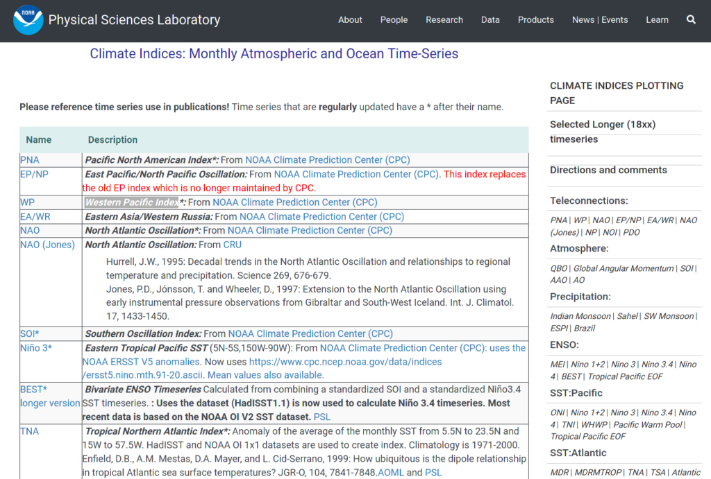
So it is a simple 2-column table, with the 1 column showing the names of the climate indices, and the 2nd some descriptions for each. In each row, the name in the 1st column is also a hyperlink linking to the data file in csv format. And there are 43 such rows.
The first step would be to fetch the contents of the page, we do this
using the built-in requests module of Python.
Then parse the returned contents using BeautifulSoup like so:
import requests
PAGE_URL = 'https://psl.noaa.gov/data/climateindices/list/'

# Getting page HTML through request
page = requests.get(PAGE_URL)
# Parsing content using beautifulsoup
soup = BeautifulSoup(page.content, 'html.parser')
Then I used the Inspect Elements function of my browser to help me locate various elements of the webpage. I use firefox, which allows me to call Inspect Elements by right-clicking on the page. Any modern browser should have such a functionality. After doing that, the browser displays this new interface at the bottom:
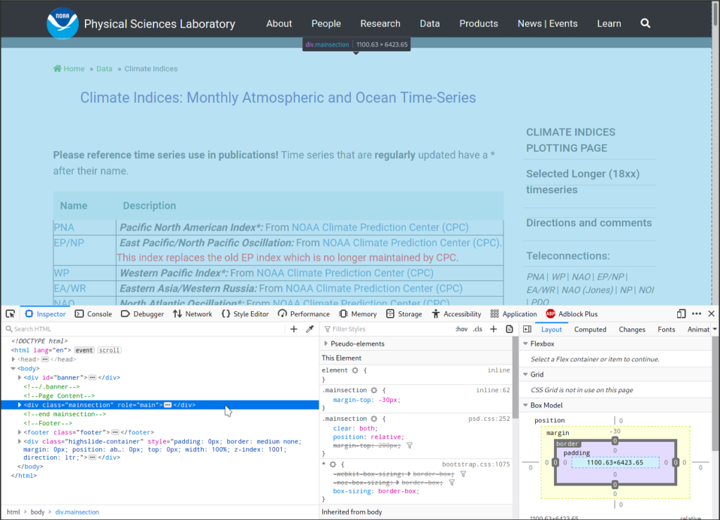
Also note that when I put the cursor at a line in the Inspector
window, the corresponding element in the displayed webpage gets
highlighted in cyan. The above screenshot shows the highlighted
element is a div with class name "mainsection".
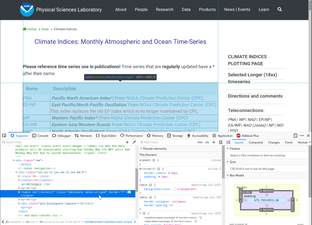
To locate the table, I expand the div tag by clicking on the grey
triangle icon on the left, and mousing over lines to see which part of
the page gets highlighted. Not surprisingly, the correct tag is a
table, see screenshot below:
To get this table from our parsed page:
# Get the big table in the page
table = soup.select('table')[0].find('tbody')
The [0] indexing is because there is only 1 table in the page, so we get
the 1st one out from a list returned by soup.select('table').
And the .find('tbody') part returns the body of the table, excluding
the header part.
By repeating the same method (mousing over things in the Inspector window) and printing things out in the Python interpreter, I arrived at the following snippet that parses the table, row by row:
# Parse table rows
table_list = []
for ii, rowii in enumerate(table.find_all('tr')):
    colsii = rowii.find_all('td')
    nameii = colsii[0].get_text().strip()
    urlii = colsii[0].find('a').get('href')
    descripii = colsii[1].get_text()
    desc_urlsii = [aii.get('href') for aii in colsii[1].find_all('a')]
    desc_urlsii = '\n'.join(
        [dii for dii in desc_urlsii if dii is not None])

    dataii = [ii, nameii, urlii, descripii, desc_urlsii]
    table_list.append(dataii)
To give some examples, below is the first 2 rows in the table_list
list:
>>> table_list[0]
[0, 'PNA', '/data/correlation/pna.data', '\xa0Pacific North American Index*:\nFrom NOAA Climate Prediction Center (CPC)', 'https://www.cpc.ncep.noaa.gov/data/teledoc/telecontents.shtml']
>>>
>>> table_list[1]
[1, 'EP/NP', '/data/correlation/epo.data', '\xa0East Pacific/North Pacific Oscillation:\nFrom NOAA Climate Prediction Center (CPC). This index replaces the old EP index which is no longer maintained by CPC.', 'https://www.cpc.ncep.noaa.gov/data/teledoc/telecontents.shtml']
Step-2: download the data and save to disk
The next step would be to iterate through the table rows, and download the data for each.
OUTPUTDIR = '/home/guangzhi/datasets/climate_indices'
for rowii in table_list:
    fetchData(rowii, OUTPUTDIR)
Each row in rowii is a Python list, containing:
- row id, e.g.
0, - name of the climate index, e.g.
'PNA', - (relative) url attached to the index name, e.g.
'/data/correlation/pna.data'. - descriptions in column 2 of the table,
- urls appeared in the descriptions.
The 3rd element in each rowii is the relative url of the data file.
Prepending it with
'https://psl.noaa.gov/' gives the absolute url. Then we can either
use requests.get() to fetch the data, or call wget as an
external command to download the data. We will be using the former here.
Code of the fetchData() function:
def fetchData(row, outputdir):
    '''Fetch data of a climate index, save to netCDF format

    Args:
        row (list): info about a climate index:
            [id, name, data_url, descriptions, urls_in_descriptions].
        outputdir (str): folder to save outputs.
    Returns:
        rec (int): 0 is run successfully.
    '''

    ii, nameii, urlii, descripii, desc_urlsii = row
    print('\n# <download_climate_indices>: Processing:', nameii)

    absurlii = 'https://psl.noaa.gov/' + urlii
    filenameii = os.path.split(urlii)[1]
    abbrii = os.path.splitext(filenameii)[0]
    abbrii = abbrii.replace('/', '-')
    abbrii = abbrii.replace('\\', '-')

    #-------save each climate index in a separate subfolder---
    subfolderii = os.path.join(outputdir, abbrii)

    if not os.path.exists(subfolderii):
        os.makedirs(subfolderii)

    #--------------Get data in csv format--------------
    abspathii_data = os.path.join(subfolderii, filenameii)
    dataii = requests.get(absurlii).text
    print('Fetched data from url:', absurlii)
    print('Writing data to file:', abspathii_data)
    with open(abspathii_data, 'w') as fout:
        fout.write(dataii)

    # ----------------Write readme----------------
    descripii = descripii + '\n\nLinks:\n' + desc_urlsii
    abspathii_dsc = os.path.join(subfolderii, 'readme.txt')
    print('Writing readme to file:', abspathii_dsc)
    with open(abspathii_dsc, 'w') as fout:
        fout.write(descripii)

    # ------------------Convert to nc------------------
    convert2NC(abspathii_data, subfolderii, abbrii, isplot=PLOT)

    return
So after a bit of house-keeping, creating sub-folders etc., the line
dataii = requests.get(absurlii).text
gets the data, which are saved in a uniform csv format. Scroll to the bottom of the page you will see the format description:
 year1 yearN
year1 janval febval marval aprval mayval junval julval augval sepval octval novval decval
year2 janval febval marval aprval mayval junval julval augval sepval octval novval decval
...
yearN janval febval marval aprval mayval junval julval augval sepval octval novval decval
  missing_value
The data are then saved to disk using:
with open(abspathii_data, 'w') as fout:
    fout.write(dataii)
After that, we also save the descriptions into an readme.txt file:
descripii = descripii + '\n\nLinks:\n' + desc_urlsii
abspathii_dsc = os.path.join(subfolderii, 'readme.txt')
print('Writing readme to file:', abspathii_dsc)
with open(abspathii_dsc, 'w') as fout:
    fout.write(descripii)
Step-3: convert to netCDF format and create a plot
The conversion to netCDF format and plot creation are done in the
convert2NC() function:
def convert2NC(abpath_in, outputdir, vid, isplot=True):
'''Convert csv data to nc format, save to disk and optionally plot
Args:
abpath_in (str): absolute path to the csv file.
outputdir (str): folder path to save outputs.
vid (str): id of variable. E.g. 'pna', 'npo'.
Keyword Args:
isplot (bool): create time series plot or not.
Returns:
rec (int): 0 is run successfully.
'''
data, years, missing, descr = readCSV(abpath_in)
data_ts = data.flatten()
data_ts = np.where(data_ts == missing, np.nan, data_ts)
timeax = createMonthlyTimeax('%04d-%02d-01' % (years[0], 1),
'%04d-%02d-01' % (years[-1], 12))
# --------Save------------------------------------
file_out_name = '%s_s_m_%d-%d_noaa.nc' % (vid, years[0], years[-1])
abpath_out = os.path.join(outputdir, file_out_name)
print('\n### <convert2nc>: Saving output to:\n', abpath_out)
with Dataset(abpath_out, 'w') as fout:
#-----------------Create time axis-----------------
# convert datetime to numbers
timeax_val = date2num(timeax, 'days since 1900-01-01')
fout.createDimension('time', None)
axisvar = fout.createVariable('time', np.float32, ('time',), zlib=True)
axisvar[:] = timeax_val
axisvar.setncattr('name', 'time')
axisvar.setncattr('units', 'days since 1900-01-01')
#-------------------Add variable-------------------
varout = fout.createVariable(vid, np.float32, ('time',), zlib=True)
varout.setncattr('long_name', '%s index' % vid)
varout.setncattr('standard_name', '%s index' % vid)
varout.setncattr('title', descr)
varout.setncattr('units', '')
varout[:] = data_ts
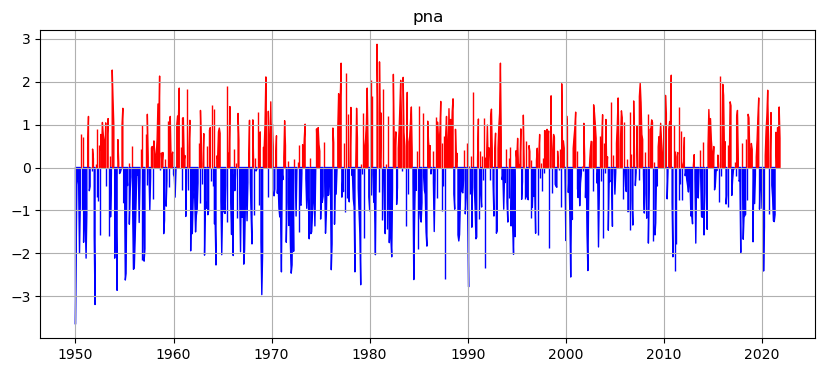
# -------------------Plot------------------------
if isplot:
import matplotlib.pyplot as plt
figure, ax = plt.subplots(figsize=(10, 4))
ts_pos = np.where(data_ts >= 0, data_ts, np.nan)
ts_neg = np.where(data_ts < 0, data_ts, np.nan)
ax.fill_between(timeax, ts_pos, y2=0, color='r')
ax.fill_between(timeax, ts_neg, y2=0, color='b')
ax.grid(True)
ax.set_title(vid)
# ----------------- Save plot------------
plot_save_name = '%s_timeseries' % vid
plot_save_name = os.path.join(outputdir, plot_save_name)
print('\n# <download_climate_indices>: Save figure to', plot_save_name)
figure.savefig(plot_save_name+'.png', dpi=100, bbox_inches='tight')
figure.savefig(plot_save_name+'.pdf', dpi=100, bbox_inches='tight')
return
Firstly, we read the csv data file and save relevant information in their correct formats. This is done in
data, years, missing, descr = readCSV(abpath_in)
where:
datais anndarray, containing the climate index values as floats.yearsis an array of integers, containing the year numbers of the index, e.g.[1948, 1949, ..., 2020].missingis a single float denoting missing values in the data, e.g.-99.9.descris a string, containing some additional information about the data provided as the last few lines in the csv file.
Here is the readCSV() function:
def readCSV(abpath_in):
    '''Read time series data in csv format

    Args:
        abpath_in (str): absolute path to csv file.
    Returns:
        data (ndarray): 2D array of floats, shape (n_years, 12).
        years (ndarray): 1d array of ints, years.
        missing (float): missing value in <data>.
        desc (str): description texts at the end of the csv data file.
    '''

    data = []
    years = []
    descr = []
    end_data = False
    with open(abpath_in, 'r') as fin:
        n = 0
        while True:
            line = fin.readline()
            if len(line) == 0:
                break
            if n == 0:
                n += 1
                continue  # skip 1st row
            line_s = line.split()
            if not end_data:
                if len(line_s) < 12:  # end of data
                    missing = float(line_s[0])
                    end_data = True
                else:
                    years.append(int(line_s[0]))
                    data.append([float(ii) for ii in line_s[1:]])
            else:
                descr.append(line.strip())
            n += 1

    years = np.array(years).astype('int')
    data = np.array(data).astype('float')
    desc = '. '.join(descr)

    return data, years, missing, desc
To create a proper netCDF data file that is self-explanatory, we also need to map the data onto a time axis.
All the climate indices are provided as monthly values, so we create the time axis by specifying a beginning month and an ending one:
timeax = createMonthlyTimeax('%04d-%02d-01' % (years[0], 1),
	'%04d-%02d-01' % (years[-1], 12))
The createMonthlyTimeax() function shown below generates a time axis
array with monthly intervals (NOTE that we use calendar month
intervals here, not the number of days between consecutive months):
def createMonthlyTimeax(t1, t2):
    '''Create monthly time axis from begining to finishing time points (both included).

    Args:
        t1, t2 (str): time strings in format %Y-%m-%d
    Returns:
        result (list): list of datetime objs, time stamps of calendar months
            from t1 to t2 (both included).
    '''

    t1dt = datetime.strptime(t1, '%Y-%m-%d')
    t2dt = datetime.strptime(t2, '%Y-%m-%d')
    result = []
    cur = t1dt
    dt = 0
    while cur <= t2dt:
        result.append(cur)
        dt += 1
        cur = datetime.strptime('%04d-%02d-01' %
                                (t1dt.year + dt // 12, t1dt.month + dt % 12),
                                '%Y-%m-%d')

    return result
The netCDF data saving and plotting parts are fairly straightforward.
Below gives a screenshot showing the contents
of the pna subfolder:
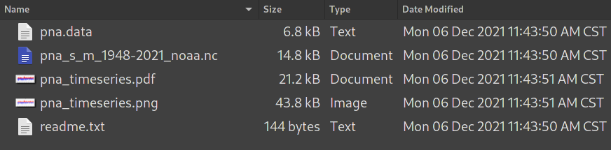
pna sub folder.pna.datais the original csv data file.pna_s_m_1948-2021_noaa.ncis the converted netCDF file.pna_timeseries.pdfand.pngare time series plots, in PDF and PNG formats.readme.txtcontains the descriptions of the climate index, in the 2nd column of the web page.
Here is the pna_timeseries.png: