Table of Contents
1 What’s this about?
Intersection-Over-Union (IoU) is a commonly used tool in object detection tasks in computer vision. It can be used to remove duplicate predictions in the Non-Maximum Suppression (NMS) process, or as a metric to gauge the model performance.
IoUs between unoriented boxes is relatively easy to compute. I have that covered in Create YOLOv3 using PyTorch from scratch (Part-4).
However, when the boxes are allowed to have arbitrary rotations, it becomes a bit tricky to compute their IoU. Depending on their positional configurations, there can be different number of intersecting points between a pair of boxes, and consequently affecting how their intersection area should be computed.
This post shows a method to compute the approximate IoU between 2 oriented 2D boxes.
It is based on a modified version of Signed Distance Function (SDF) for oriented 2D boxes, using L1-norm as distance measure, instead of the convention Euclidean (L2-norm) distance. This SDF-L1 definition is detailed in my previous post Signed distance function to oriented 2D boxes.
The following parts will cover:
- Formulation of the problem
- Derivation of the approximate IoU algorithm
- Python implementation
- Some discussions
2 Formulation of the problem
First introduce a few notations:
- \(A^*\): ground truth box, and so its area.
- \(A’\): prediction box, and so its area.
One way to formulate the IoU is using the intersection area \(I\):
\begin{equation} \label{org522c30c} IoU \equiv \frac{I}{U} = \frac{I}{A^* + A’ – I} \end{equation}This formulation would require the computation of intersection area \(I\).
Another equivalent formulation is to use the union area \(U\):
\begin{equation} \label{org04b4f0b} IoU \equiv \frac{I}{U} = \frac{A^* + A’ – U}{U} = \frac{A^* + A’}{U} – 1 \end{equation}We will take the latter union-based formulation.
3 Derivation of the approximate IoU algorithm
3.1 Compute the union area
Notice that when the 2 boxes are too far apart such that there is no intersection, the union area is just the sum of the 2 areas.
When the 2 boxes do have intersections, the union area is the target/ground-truth box area, plus some extra bits from the predicted box that is outside of the target box, i.e. the area of \(A’ \setminus A^*\). This is represented as blue shading in the schematic in Figure 1.
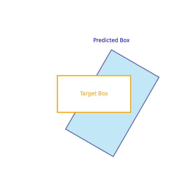
Figure 1: Schematic of IoU computation between oriented boxes.
Denote this \(A’ \setminus A^*\) area as \(A_{extra}\). Then we have an expression for the union area \(U\):
\begin{equation} \label{orgfd579eb} U = \begin{cases} A^* + A’ & I = 0\\ A^* + A_{extra} & I > 0 \end{cases} \end{equation}It is relatively easy to determine when \(I\) is guaranteed to be 0. We can compare the center distance between the 2 boxes with the sum of their diagonal lengths divided by 2. Even when the test has been too conservative (the 2 boxes have no intersection, when their center distance is smaller than half of the diagonal sum), the approximate algorithm still works.
Now the problem reduces to how to compute \(A_{extra}\).
3.2 Approximate \(A_{extra}\) using SDF-L1
Notice that the area of \(A_{extra}\) is formed by points along the edges of the blue prediction box, and the edge of the orange target box (see Figure 1).
How far away the individual points along the blue edges can be quantified using SDF to the target box.
However, the conventional definition of SDF to oriented boxes renders contour lines that have rounded corners. See Figure 2a (see also Figure 2a in Signed distance function to oriented 2D boxes). Such rounded corners are not helpful to our task of quantifying \(A_{extra}\).
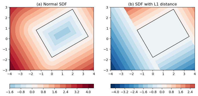
Figure 2: SDF to a box centered at (1, 0.5) with 30 degree rotation. (a) normal SDFs. (b) SDFs with L1-norm distance. The box itself is drawn as black.
This is where the modified version – SDF-L1 – comes into the equation. By replacing L2-norm distances with L1-norm, we remove the rounded corners from the distance contours. See Figure 2b.
This L1-norm formulation makes it easy to determine how far away an outside point \(P\) is from the infinite line along which the target box’s right edge is located, if \(P\) is located to the right of the target box.
Similarly, if \(P\) is located above the target, within the span of the target’s width, the distance between \(P\) and the target box is the distance between \(P\) and the infinite line that the top edge is located.
Having got the perpendicular distances between points along the prediction box’s edges, \(A_{extra}\) can then be approximated by sub-dividing the prediction box’s edges and forming a series of trapezoids. The heights of the trapezoids are the SDF-L1 values, and the bases are the small “lateral” steps \(dx\), or \(dy\), depending on whether the SDF-L1 values are horizontal or vertical.
Figure 3 below shows the process of sub-dividing the edge formed by vertices 1 and 2 of the prediction box, into 13 evenly spaced segments.
The SDF-L1 field is drawn as (faded) contours in the background. The 2 vertical grey lines show the left-mid-right segmentation of the SDF-L1 field. Therefore, part of the 1-2 edge falls into the mid section, where SDF-L1 have negative y- values, and the “lateral” steps are \(dx\). And part of the 1-2 edge falls into the right section, where SDF-L1 have positive x- values, and the “lateral” steps take \(dy\). The total area of these trapezoids can be approximated by 2 integrations \(\int SDF_x dy + \int SDF_y dx\).
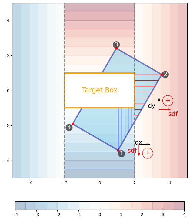
Figure 3: Sub-division of the edge formed by vertices 1 and 2 of the prediction box (blue) into 13 evenly spaced segments. At each bin edge, a perpendicular line is drawn from the sub-division point along the edge, to the edge of the target box (orange). The perpendicular line is horizontal, if the line falls into the right- section. In such cases, the SDF values are positive, and the widths of the bins take \(dy\), as shown by the red and black arrows. The perpendicular line is vertical, if the line falls into the mid- section, and the SDF values are negative, and bin widths take \(dx\), as shown by the blue and black arrows. The left-, mid- and right- sections are denoted by the 2 vertical grey lines. SDF-L1 field is drawn as faded color contours in the background.
In Figure 3, we covered part of the \(A_{extra}\) area by sub-dividing the 1-2 edge and integrating the SDF-L1 values. Now do the similar for the 2-3 edge, shown in Figure 4.
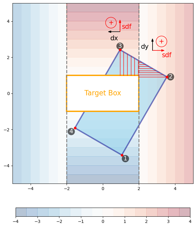
Figure 4: Similar as Figure 3 but for the edge between vertices 2 and 3.
Again, part of the SDF-L1 heights are in the mid- section, where SDF values are positive and vertical, and part of the SDF-L1 heights are in the right- section, where SDF values are positive and horizontal. Then repeat for the 3-4 edge, shown in Figure 5.
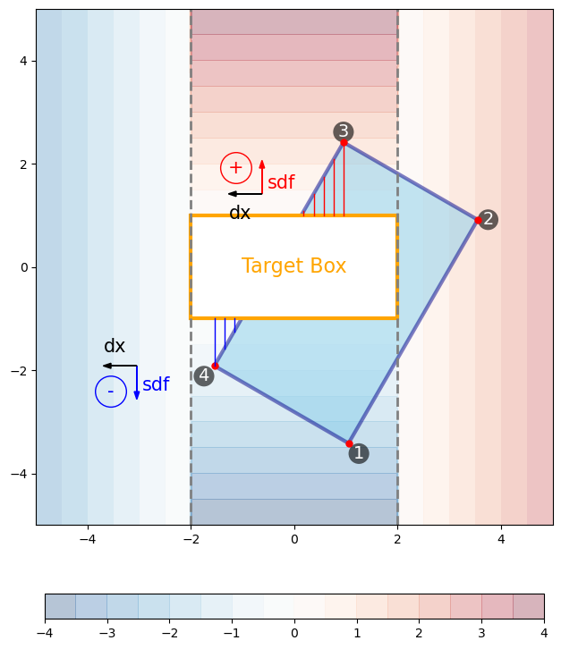
Figure 5: Similar as Figure 3 but for the edge between vertices 3 and 4.
Notice that SDF-L1 is not defined inside the box, so there are no SDF-L1 heights when the target box cuts into the prediction box, thereby we only account for the area outside of the target box.
Also notice that we are giving the SDF-L1 values signs (red color for positive, blue for negative). Why using signed values for the computation of area?
This is because sometimes there will be regions whose area get integrated more than once. For instance the lower-left triangle shown by blue SDF-L1 heights in Figure 5. This same triangle will also be covered when we take the integration process along the 4-1 edge, shown in Figure 6.
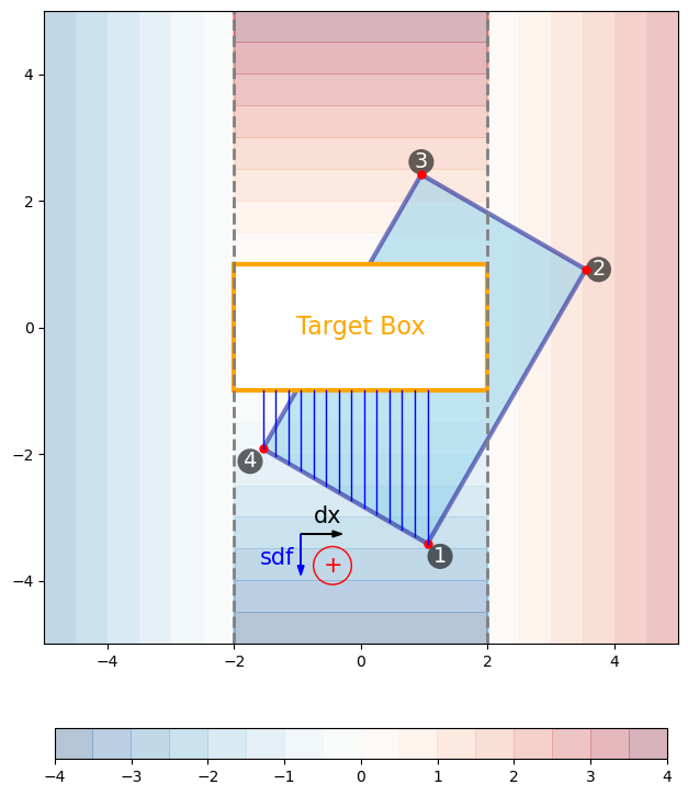
Figure 6: Similar as Figure 3 but for the edge between vertices 4 and 1.
Therefore, we need some kind of mechanism to offset such double-counting. It turns out that by giving the trapezoid heights and bases signed values (effectively making them into vectors), and using cross product to compute signed areas, we can effectively get rid of the double-counted areas as we move around the box edge.
Now refer back to Figure 3–6 and check out the \(+\) or \(-\) signs shown next to the SDF-L1 and \(dx/dy\) vectors. Those are the signs of the cross products between those vector pairs, using the right-hand rule. There is only 1 cross product that has a minus sign, and that appears in the lower-left triangular region when we integrate the 3-4 edge. Notice that this same triangular area is offset by a positive areal integration, when we integrate along the 4-1 edge.
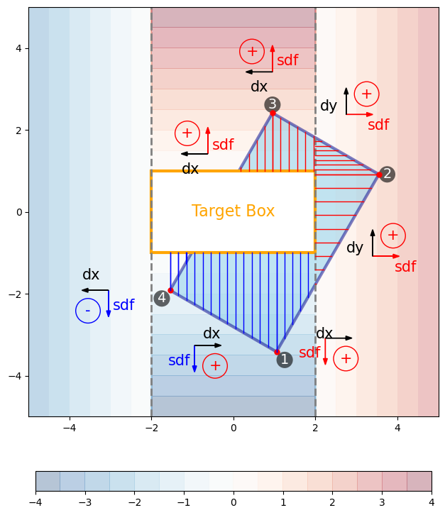
Figure 7: Similar as Figure 3 but for all 4 edges.
Figure 7 shows the entire integration process after finishing a whole loop around the prediction box, and the total integrated area gives an approximate to \(A_{extra}\). Lastly, the approximate IoU can be computed by substituting \(A_{extra}\) into Equation \eqref{orgfd579eb}, then Equation \eqref{org04b4f0b}.
Lastly, let’s call this area-finding method signed area function (SAF).
4 Python implementation
4.1 SDF-L1 between oriented boxes
The function sdf_obox_l1() for computing SDF-L1 values to an oriented box is given
in Signed distance function to oriented 2D boxes.
4.2 Convert oriented box to 4-polygon
This is a helper function that converts an oriented box encoded in
[x_center, y_center, width, height, angle] format into a 4-polygon:
def obbox2poly(xc, yc, w, h, theta, close=False):
    '''Convert oriented box to 4-polygon, single box
    Order: bottom-right, top-right, top-left, bottom-left'''

    cos, sin = np.cos(theta), np.sin(theta)
    rot = np.array([[cos, -sin], [sin, cos]])
    center = np.c_[xc, yc]
    corner_xy = np.array([
        [w/2, -h/2],
        [w/2,  h/2],
        [-w/2,  h/2],
        [-w/2, -h/2]])
    corner_xy = corner_xy.dot(rot.T)
    corner_xy = center + corner_xy

    if close:
        return np.r_[corner_xy, corner_xy[0:1]]
    else:
        return corner_xy
4.3 SAF between 2 oriented boxes
The following function saf_obox2obox() computes \(A_{extra}\):
def saf_obox2obox(pred_box, gt_box, n_samples=40):
    '''Signed area difference formed between a single pair of predition and target boxes

    Args:
        pred_box (ndarray): predition box in [xc, yc, w, h, angle].
        gt_box (ndarray): reference box in [xc, yc, w, h, angle].
    Keyword Args:
        n_samples (int): number of points to sample along box perimeter.
    Return:
        saf (float): mean sdf difference, i.e. the area of <gt_box> diff <pred_box>.
    '''

    pred_poly = obbox2poly(*pred_box, close=True)
    angle = gt_box[-1]
    rot = np.array([[np.cos(angle), -np.sin(angle)],
                    [np.sin(angle),  np.cos(angle)]])
    saf = 0
    for (x1, y1), (x2, y2) in zip(pred_poly[:-1], pred_poly[1:]):
        pii = np.linspace([x1, y1], [x2, y2], n_samples, True)
        sdfii, sdfxyii = sdf_obox_l1(pii,
            gt_box[0],
            gt_box[1],
            gt_box[2],
            gt_box[3],
            gt_box[4],
            True)
        pii = pii.dot(rot)
        dxyii = np.gradient(pii, axis=0)
        sdfii = np.cross(sdfxyii, dxyii)
        saf += sdfii.sum()

    return saf
A few points to note:
- We take a full loop around the 4 edges of the prediction box, for
each edge, the starting point is
(x1, y1)and the ending point(x2, y2). - Then we evenly sample the edge into
n_samplesintervals. - For those sampled points, compute their SDF-L1 values using
sdf_obox_l1(), and return also the x- and y- components insdfxyii. - In the schematics in Figure 3–7, the target box (and
therefore the SDF-L1 field) has no rotation. In the general case
where the target box is oriented (as in Figure 1), we need to
do an counter-rotation so the target box is not oriented. This is
done in
pii = pii.dot(rot). - After the rotation, the \(dx\) and \(dy\) values are computed using
np.gradient(pii, axis=0). - Finally, we compute the signed area using
np.cross(sdfxyii,
  dxyii)
, and integrate that to get the finalsaf.
4.4 Some examples
Time for some test runs.
To validate the algorithm, I use the shapely module to compute the
ground truth union area of 2 boxes, and compare that with the
approximate solution. Code below:
from shapely.geometry import Polygon
import numpy as np
import matplotlib.pyplot as plt

figure = plt.figure(figsize=(10, 5))
# example 1
# target box
xc = 2
yc = 1
w = 4
h = 2.5
angle = 30/180*np.pi
gt_box = [xc, yc, w, h, angle]
gt_poly = obbox2poly(*gt_box, False)
gt_poly_sp = Polygon(gt_poly)

# prediction box
box = [4, 3, 4, 5, 145/180*np.pi]
box_poly = obbox2poly(*box, False)
box_poly_sp = Polygon(box_poly)

aa = saf_obox2obox(box, gt_box, 20)
union = gt_poly_sp.union(box_poly_sp).area
union_hat = gt_box[2] * gt_box[3] + aa
print('Union area:', union)
print('Union hat area:', union_hat)

ax = figure.add_subplot(1, 2, 1)
gt_poly = obbox2poly(*gt_box, True)
box_poly = obbox2poly(*box, True)
ax.plot(gt_poly[:, 0], gt_poly[:, 1], 'r-', label='Target')
ax.plot(box_poly[:, 0], box_poly[:, 1], 'b-', label='Prediction')
ax.set_aspect('equal')
ax.set_title('true union: %.3f, approx union: %.3f' % (union, union_hat))
ax.legend()

# example 2
# target box
xc = 2.2
yc = 1
w = 4
h = 2.5
angle = 30/180*np.pi
gt_box = [xc, yc, w, h, angle]
gt_poly = obbox2poly(*gt_box, False)
gt_poly_sp = Polygon(gt_poly)

# prediction box
box = [-2, 3, 4, 5, 45/180*np.pi]
box_poly = obbox2poly(*box, False)
box_poly_sp = Polygon(box_poly)

aa = saf_obox2obox(box, gt_box, 20)
union = gt_poly_sp.union(box_poly_sp).area
union_hat = gt_box[2] * gt_box[3] + aa
print('Union area:', union)
print('Union hat area:', union_hat)

ax = figure.add_subplot(1, 2, 2)
gt_poly = obbox2poly(*gt_box, True)
box_poly = obbox2poly(*box, True)
ax.plot(gt_poly[:, 0], gt_poly[:, 1], 'r-', label='Target')
ax.plot(box_poly[:, 0], box_poly[:, 1], 'b-', label='Prediction')
ax.set_aspect('equal')
ax.set_title('true union: %.3f, approx union: %.3f' % (union, union_hat))
ax.legend()

figure.show()
The output figure:
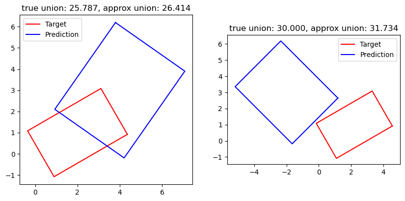
Figure 8: 2 examples of approximated union area formed by a target box (red) and prediction box (blue).
It is seen that the approximate solution using 20 sub-division steps for each edge is slightly bigger than the ground truth. This is because our integration of the trapezoid areas is not adjusting for the triangular top, but instead using rectangular approximations.
It is also noticed that when the 2 boxes have no intersection (Figure 8b), the method works as well.
4.5 Vectorized versions
In practice, one often needs to deal with multiple pairs of targets and predictions. It would be much more efficient to vectorize the computations.
4.5.1 Vectorized obbox2poly()
Convert an array of oriented boxes in
[x_center, y_center, width, height, angle] format into 4-polygons:
def obbox2poly2(oboxes, close=False):
    '''Convert oriented box to 4-polygon, multiple boxes

    Args:
        oboxes (ndarray): (n, 5) oriented boxes, [xc, yc, w, h, angle].

    Order: bottom-right, top-right, top-left, bottom-left'''

    center, w, h, theta = np.split(oboxes, [2, 3, 4], axis=1)
    cos, sin = np.cos(theta), np.sin(theta)
    rot = np.concatenate([cos, -sin, sin, cos], axis=1).reshape(-1, 2, 2)
    p1 = np.concatenate([w/2, -h/2], 1)
    p2 = np.concatenate([w/2, h/2], 1)
    p3 = np.concatenate([-w/2, h/2], 1)
    p4 = np.concatenate([-w/2, -h/2], 1)

    p1 = (rot * p1[:, None, :]).sum(-1)
    p2 = (rot * p2[:, None, :]).sum(-1)
    p3 = (rot * p3[:, None, :]).sum(-1)
    p4 = (rot * p4[:, None, :]).sum(-1)

    corner_xy = np.stack([p1, p2, p3, p4], axis=1)
    corner_xy = center[:, None, :] + corner_xy

    if close:
        return np.r_[corner_xy, corner_xy[0:1]]
    else:
        return corner_xy
4.5.2 Vectorized saf_obox2obox()
Deals with the computation of pairwise \(A_{extra}\) between n
predictions and m targets:
def saf_obox2obox_vec(pred_oboxes, target_oboxes, n_samples=40):
    '''Signed area difference between 2 sets of oriented boxes, vectorized

    Args:
        pred_oboxes (ndarray): prediction oboxes, in shape (n, 5). Columns: [xc, yc, w, h, angle].
        target_oboxes (ndarray): target oboxes, in shape (m, 5). Columns: [xc, yc, w, h, angle].
    Keyword Args:
        n_samples (int): number of samples along each edge.
    Returns:
        saf (ndarray): (n, m) array, mean saf between pairs of pred/target.
    '''

    # from [xc, yc, w, h, angle] -> [x1,y1, x2,y2, x3,y3, x4,y4]
    poly = obbox2poly2(pred_oboxes)
    factors2 = np.arange(n_samples) / n_samples
    factors1 = 1. - factors2

    center = target_oboxes[:, :2]          # [m, 2]
    cos = np.cos(target_oboxes[:, -1])     # [m,1]
    sin = np.sin(target_oboxes[:, -1])     # [m,1]
    saf = 0

    for i1 in range(4):
        # linearly sample n_samples points along each edge
        i2 = (i1 + 1) % 4
        p1 = poly[:, i1, :]
        p2 = poly[:, i2, :]
        pnew = p1[:, None, :] * factors1[None, :, None] +\
               p2[:, None, :] * factors2[None, :, None]
        pnew = pnew[:, None, :, :] - center[None, :, None, :]  # [n, m, n_samples, 2]

        ppx = pnew[..., 0] * cos[None, :, None] +\
              pnew[..., 1] * sin[None, :, None]  # [n, m, n_samples]
        ppy = -pnew[..., 0] * sin[None, :, None] +\
               pnew[..., 1] * cos[None, :, None]  # [n, m, n_samples]
        ppxy = np.stack([ppx, ppy], axis=3)  # [n, m, n_samples, 2]
        qqxy = np.abs(ppxy) - 0.5 * target_oboxes[None, :, None, 2:4] # [n, m, n_samples, 2]

        sign = qqxy[..., 0] > 0  # [n, m, n_samples]
        x_comp = np.maximum(qqxy[..., 0], 0) * sign * np.sign(ppxy[..., 0]) # [n, m, n_samples]
        y_comp = np.maximum(qqxy[..., 1], 0) * (1 - sign) * np.sign(ppxy[..., 1])

        dx = np.gradient(ppx, axis=-1)  # [n, m, n_samples]
        dy = np.gradient(ppy, axis=-1)  # [n, m, n_samples]

        safii = x_comp * dy - y_comp * dx
        saf = saf + safii.sum(axis=-1)

    return saf
5 Summary and some discussions
This post shows an approximation method to compute the IoU between oriented 2D boxes.
The problem is formulated into a search for the union area of the 2 boxes, and then a search for the area of the relative component of target box in prediction box: \(A_{extra} \equiv A’ \setminus A^*\).
\(A_{extra}\) is approximated by sub-dividing it into a series a small bins, and integrating the bin areas using SDF-L1 values as heights, and small \(dx\) or \(dy\) steps as bases.
SDF-L1 is a modification of the conventional SDF by replacing L2-norm distances with L1-norm distances. Doing this removes the rounded corners in the SDF field.
The double-counted areas during the integration process as we take a full loop around the 4 edges are offset by using signed areas, achieved using cross products between the SDF-L1 vectors and the edge segment vectors. This is why the SDF-L1 values have signs.
Some advantages of this approach:
- Can be easily vectorized for multiple predictions and targets.
- Can control the trade-off between accuracy and efficiency, by adjusting the sub-division number.
Some limitations of this approach:
- Gives approximated solution.
- Tends to overestimate the union area.
Created: 2022-09-28 Wed 11:38


