Table of Contents
1. Overview
This is Part-4 of the series on building a YOLOv3 model from scratch.
Here is an overview of the series:
- Understand the YOLO model.
- Build the model backbone.
- Load pre-trained weights.
Get the tools ready: this post.
Before getting into the training part, it might be helpful to first get some utilities ready, including the codes to compute IoU (Intersection-Over-Union), NMS (Non-Maximum suppression) and mAP (mean Average Precision).
- Training data preparation.
- Train the model.
2. Intersection-Over-Union (IoU)
2.1. Concept
IoU is a common metric in object detection tasks. It is the ratio of, as its name suggests, intersection over union. Figure 1 gives an illustration.
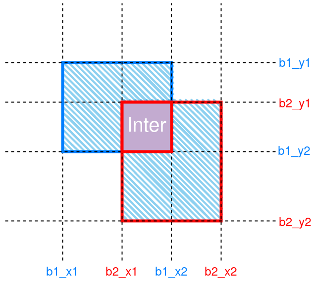
Figure 1: Schematic of IoU between 2 boxes. The intersection region is labeled “Inter”. Union is denoted by hatching.
2.2. Python code
The implementation is also fairly simple. Code first:
def compute_IOU(bbox1, bbox2, x1y1x2y2=False, change_enclose=False):
    '''Compute IoU of 2 groups of bounding boxes

    Args:
        bbox1 (ndarray or tensor): bounding box 1, in either [x_center, y_center, w, h]
            format, or [x1, y1, x2, y2] format.
        bbox2 (ndarray or tensor): bounding box 2, in either [x_center, y_center, w, h]
            format, or [x1, y1, x2, y2] format.
    Keyword Args:
        x1y1x2y2 (bool): If True, assumes bbox1 and bbox2 are in [x1, y1, x2, y2] format.
        change_enclose (bool): If True, when either box is enclosed by the other,
            change iou to 1.
    Returns:
        iou (ndarray or tensor): intersection over union ratios.
    '''

    if not x1y1x2y2:
        bbox1 = to_x1y1x2y2(bbox1)
        bbox2 = to_x1y1x2y2(bbox2)

    b1x1, b1y1, b1x2, b1y2 = bbox1[:,0], bbox1[:,1], bbox1[:,2], bbox1[:,3]
    b2x1, b2y1, b2x2, b2y2 = bbox2[:,0], bbox2[:,1], bbox2[:,2], bbox2[:,3]

    if isinstance(bbox1, torch.Tensor):
        # intersection coordinates
        inter_x1 = torch.max(b1x1, b2x1)
        inter_x2 = torch.min(b1x2, b2x2)
        inter_y1 = torch.max(b1y1, b2y1)
        inter_y2 = torch.min(b1y2, b2y2)

        # intersection area
        inter = torch.clamp(inter_x2 - inter_x1, 0, None) * torch.clamp(inter_y2 - inter_y1, 0, None)
    else:
        # intersection coordinates
        inter_x1 = np.maximum(b1x1, b2x1)
        inter_x2 = np.minimum(b1x2, b2x2)
        inter_y1 = np.maximum(b1y1, b2y1)
        inter_y2 = np.minimum(b1y2, b2y2)

        # intersection area
        inter = np.clip(inter_x2 - inter_x1, 0, None) * np.clip(inter_y2 - inter_y1, 0, None)

    w1, h1 = (b1x2 - b1x1) , (b1y2 - b1y1)
    w2, h2 = (b2x2 - b2x1) , (b2y2 - b2y1)
    area1 = w1 * h1
    area2 = w2 * h2

    # union area
    union = area1 + area2 - inter

    # iou
    iou = inter / (union + 1e-7)

    if change_enclose:
        # check if box1 inside box2
        idx = abs(area1 / (area2 + 1e-6) - iou) <= 1e-3
        iou[idx] = (inter / (area1 + 1e-6))[idx]

        # check if box2 inside box1
        idx = abs(area2 / (area1 + 1e-6) - iou) <= 1e-3
        iou[idx] = (inter / (area2 + 1e-6))[idx]

    return iou
Some points to note:
- We put this
compute_IOU()function in theutils.pyscript in theYOLOv3_pytorchproject folder. For a structure of the folder, refer back to the Create the Darknet-53 model section of part-2. - We assume the input arguments
bbox1andbbox2are bounding boxes as either numpy arrays or torch tensors, and have columns of [xcenter, ycenter, width, height], or [x1, y1, x2, y2]. Sometimes, a small bounding box may be entirely enclosed by a larger one, then the IoU will be the areal ratio between the 2, and could be a fairly small number. This may cause trouble when doing the NMS filtering. We will see why it is an issue in the next section. But to prevent such an issue, we manually change the IoU values of such cases to a number close to
1, if thechange_encloseinput argument is set toTrue:if change_enclose: # check if box1 inside box2 idx = abs(area1 / (area2 + 1e-6) - iou) <= 1e-3 iou[idx] = (inter / (area1 + 1e-6))[idx] # check if box2 inside box1 idx = abs(area2 / (area1 + 1e-6) - iou) <= 1e-3 iou[idx] = (inter / (area2 + 1e-6))[idx]
To convert bounding boxes in [xcenter, ycenter, width, height] format to [x1, y1, x2, y2], we use a
to_x1y1x2y2()function:def to_x1y1x2y2(bbox): '''Convert from [x_center, y_center, w, h] -> [x1, y1, x2, y2] ''' x1 = bbox[:,0] - bbox[:,2] / 2 x2 = bbox[:,0] + bbox[:,2] / 2 y1 = bbox[:,1] - bbox[:,3] / 2 y2 = bbox[:,1] + bbox[:,3] / 2 if isinstance(bbox, torch.Tensor): return torch.vstack([x1, y1, x2, y2]).T else: return np.c_[x1, y1, x2, y2]
3. Non-Maximum suppression (NMS)
3.1. Concept
NMS is often used to remove duplicate predictions, where multiple similar bounding boxes are predicted around a same target. Figure 2 gives an illustration of the process.
The steps of NMS:
Sort the predictions by their confidence scores, from highest to lowest, and put them into a “waiting list”. In the example of Figure 2, we have:
box index confidence score 1 0.99 4 0.98 2 0.90 3 0.81 5 0.70 6 0.50 - Select the top-ranking bounding box (box-1), remove it from the “waiting list” and put it into the result list.
Compute IoU scores between the just selected bounding box with all remaining ones in the “waiting list”. Remove boxes with IoU scores greater than a prescribed threshold (typically 0.5) from the “waiting list”.
In the example of Figure 2, let’s assume that box-2, and -3 overlap with box-1 with
IoUs >= 0.5, so they are removed. Box-4, -5 and -6 have little to none overlap with box-1, so they stay in the “waiting list”. This makes sense since we are picking a “winner” predictor by suppressing similar competitors, but leaving those irrelevant predictors alone.- Repeat step-2 and -3 until the “waiting list” is empty.
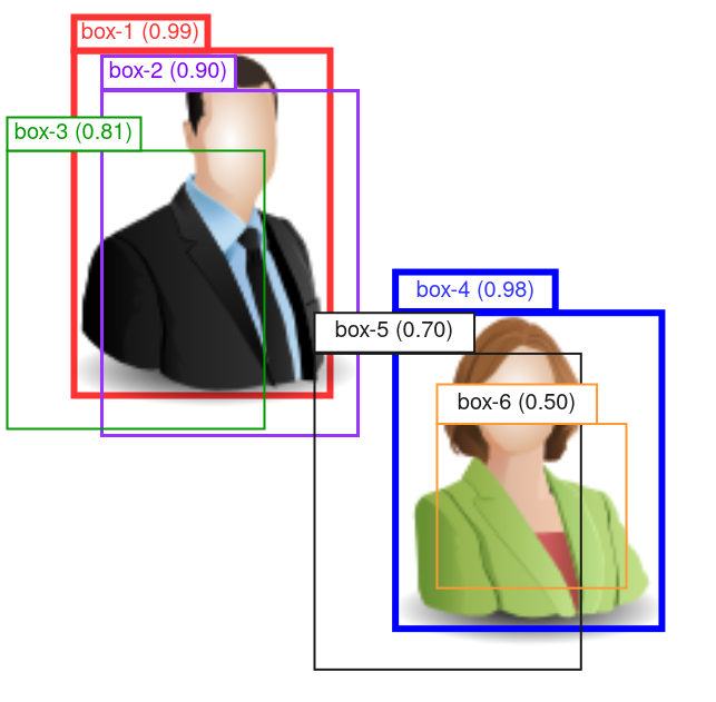
Figure 2: Schematic of the NMS process. Confidence score of each bounding box is shown in parentheses in the box label.
In the example in Figure 2, after having selected box-1 and removed box-2 and -3, we pick box-4 as the next top-ranking box. Then we compute the IoUs between box-4 with -5 and -6.
Notice that box-6 is entirely enclosed by box-4, so the “original” IoU
ratio will be fairly small, and there is a high chance that it is
below the 0.5 threshold, and thus doesn’t get removed.
That’s why when enclosing bounding boxes are detected, we manually
change the IoU to the ratio of intersection over the area of the
smaller box, which essentially gives an IoU of 1.0.
3.2. Python code for NMS()
Code first:
def NMS(predictions, conf_thres, iou_thres, verbose=True):
    '''Non-maximum suppression on predictions of a single image

    Args:
        predictions (ndarray): bbox predictions. In shape (n, 5+n_classes).
            First 5 columns are: [x_c, y_c, w, h, conf_score]. Last n_classes
            columns are classification predictions.
        conf_thres (float): filter out detections with object confidence score
            lower than this.
        iou_thres (float): float in range [0, 1]. Suppress bboxes with overlaps
            greater than this ratio.
    Returns:
        results (ndarray): filtered detections, in shape (m, 6). m is the number
            of filtered detections. Columns are: [x_c, y_c, w, h, conf_score, class_idx].
            class_idx is np.argmax(results[:,5:], axis=1).
    '''

    results = []
    conf_idx = 4

    if verbose:
        print('Number of predictions before confidence filtering:', len(predictions))

    # select by conf
    idx = predictions[:, conf_idx] >= conf_thres
    predictions = predictions[idx]
    if len(predictions) == 0:
        return results

    if verbose:
        print('Number of predictions after confidence filtering:', len(predictions))

    # conditional on objectness
    predictions[:, 5:] *= predictions[:, 4:5]

    # select by class prob. idx_box select bboxes, idx_cls select classes
    idx_box, idx_cls = np.where(predictions[:, 5:] >= conf_thres)
    boxes = predictions[idx_box, :4]
    confs = predictions[idx_box, idx_cls+5]
    clss = idx_cls[:, None]
    pred = np.c_[boxes, confs, clss]  # [m, 6]

    if verbose:
        print('Number of predictions after class prob filtering:', len(pred))
    if len(pred) == 0:
        return results

    # sort by conf
    idx = np.argsort(pred[:, conf_idx])[::-1]
    pred = pred[idx]
    # NMS
    while True:
        p1, pred = pred[0:1], pred[1:]
        results.append(p1)
        if len(pred) == 0:
            break

        # compute iou with others
        ious = compute_IOU(p1[:4], pred[:, :4], x1y1x2y2=False, change_enclose=True)
        # remove overlaps
        pred = pred[ious < iou_thres]

    results = np.vstack(results)

    return results
Some points:
- The low confident predictions are first removed by a
conf_thresthreshold. This will drastically reduced the number of candidates to go through. Recall that with an input size of416 x 416and 3 size scales, YOLOv3 outputs(52 * 52 + 26 * 26 + 13 * 13) * 3 = 10647predictions per image. With a confidence thresholding we can reduce that down to about a hundred, or even fewer, depending the chosen threshold. The classification probabilities are conditioned on objectness confidence score:
predictions[:, 5:] *= predictions[:, 4:5]
3.3. Python code for batch_NMS()
The above NMS() function works on a single image. We then create
another function that works on a batch:
def batch_NMS(predictions, conf_thres, iou_thres):
    '''Do Non-maximum suppression on a batch

    Args:
        predictions (ndarray): detection predictions, in shape (b, n, 5+n_classes).
            b: batch size, n: number of predictions.
        conf_thres (float): filter out detections with object confidence score
            lower than this.
        iou_thres (float): float in range [0, 1]. Suppress bboxes with overlaps
            greater than this ratio.
    Returns:
        results (ndarray): filtered detections for each image in the batch.
            Shape (m, 7). m is number of detections after filtering.
            Columns are: [batch_idx, x_c, y_c, w, h, conf_score, class_idx].
    '''

    results = []
    #---------------Loop through images---------------
    for ii, pii in enumerate(predictions):
        resii = NMS(pii, conf_thres, iou_thres)
        if len(resii) > 0:
            # prepend batch idx to 1st column
            resii = np.c_[np.full([len(resii), 1], ii), resii]
            results.append(resii)

    if len(results):
        results = np.vstack(results)
    return results
It simply iterates through the images in a batch, and calls NMS() on
each. If anything is remained after the filtering, we prepend it with
an extra column containing the batch indices.
4. mean Average Precision (mAP)
I personally find the concept of mAP rather confusing. I list a few references I used below:
- https://pyimagesearch.com/2022/05/02/mean-average-precision-map-using-the-coco-evaluator/
- https://towardsdatascience.com/breaking-down-mean-average-precision-map-ae462f623a52
- https://www.youtube.com/watch?v=FppOzcDvaDI
And here are another 2 that I believe are inaccurate (at least):
- https://blog.paperspace.com/mean-average-precision/
- https://www.v7labs.com/blog/mean-average-precision
The key point, I think, is how to get the Precision-Recall curve. But let’s start from the beginning.
4.1. mAP is the average of APs, and AP is parameterized on IoU threshold
mAP (mean Average Precision), is an averaged score across multiple classes. E.g. across the 80 different classes in the COCO detection dataset. For each class, we compute an AP (Average Precision), and the results of all classes are averaged to get the mAP.
The AP score is parameterized by the IoU threshold. For instance, the “traditional” way, also the way used in PASCAL VOC metric, uses a IoU threshold of 0.5. Thus computed AP is denoted as AP@IoU=0.5.
Instead of taking a single IoU=0.5 threshold, one could take
multiple IoU thresholds and average the results. For instance,
repeat the similar computations at 10 different IoU thresholds,
starting from 0.5 to 0.95, with a step of 0.05. The averaged
final result is denoted AP@[0.5:0.05:0.95]. This is the so-called
COCO primary challenge metric. But let’s leave this multiple-IoU
threshold thing to the very end.
Note that the IoU threshold here is NOT the same thing as the threshold used in the NMS process:
- The IoU threshold in the NMS process is used to flag duplicates.
- the IoU threshold for AP computation is used to flag true positive and false positive predictions.
4.2. True and false positive predictions, precision and recall
So how do we decide whether a prediction is true or false?
Recall that AP is conditioned on a specific class, so the predicted object has to be of the correct class.
Then the localization of the prediction has to be reasonably
good. This is measured by the IoU score: if the predicted bounding box
overlaps with a ground truth label of the specific class at IoU
>= IoU_threshold, then it is flagged as a true positive prediction.
Otherwise, it is a false positive prediction.
An example is given in Figure 3. The predicted boxes have gone through the NMS process, and there are 4 boxes left: box-1, -2, -7 and -8.
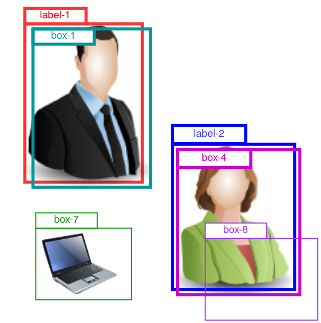
Figure 3: Demo for AP computation for the “person” class. 2 ground truth labels are given as “label-1” and “label-2”. 4 preditions are given as “box-1”, “box-4”, “box-7” and “box-8”.
Here, we are looking at the AP for the “person” class, so box-7 that predicts a laptop is irrelevant, and we ignore it.
There are 2 ground truth “person” labels in the this image. Box-1 is a close match with label-1, so it is a true positive. Similarly for box-4.
Box-8 also predicts a “person”, but by too poor a localization (IoU
with label-2 < the IoU threshold, which, for instance, was set to
0.5). So box-8 is flagged as false positive.
But how do we know box-1 should be compared against label-1, and box-8 against label-2? In fact, we compare each prediction with all labels of class “person”, and chose the best match with the highest IoU.
Then, for this image and class “person”, we have 2 true positives:
TP=2, and 1 false positive: FP=1.
So, precision and recall can be computed:
- precision:
P = TP / (TP + FP) = 2 / 3 = 0.666. - recall:
R = TP / #labels = 2 / 2 = 1.
4.3. Area Under the P-R Curve (AUC)
Precision and recall are 2 competing scores, and typically one has to scarifies one for another. Only a hypothetically ideal predictor can achieve precision = recall = 1.
To measure the combined effect of precision and recall, we can compute the Area Under the Curve (AUC), with Precision (P) on the y-axis, and Recall (R) on the x-axis. And this area is defined as the AP for this class.
So we need to first construct such a P-R curve.
Here is where I think the 2 posts I gave above are inaccurate: they seem
to suggest that one constructs a P-R curve by iterating through a range
of IoU thresholds. Doing that does give us a list of (P, R) pairs, but that
is in contradiction to the fact one can compute the AUC, and the AP
score, at a fixed IoU=0.5 threshold.
So I believe the following method is correct:
- Pick an IoU threshold level, e.g.
IoU=0.5. - Pick a class, e.g. “person”.
- Get an image been predicted, and its ground truth label. Select detections of the “person” class, and labels of the “person” class.
- Decide each of the detections is true or false positive, as done in the previous sub-section.
- Repeat 3-4 for all the images to be evaluated.
- Put results in a table like below:
| conf score (float) | TP (1 or 0) | FP (1 or 0) | Accum TP (int) | Accum FP (int) | Precision (float) | Recall (float) |
|---|---|---|---|---|---|---|
| 0.98 | 1 | 0 | 1 | 0 | 1 / 1 | 1 / N |
| 0.88 | 1 | 0 | 2 | 0 | 2 / 2 | 2 / N |
| 0.80 | 0 | 1 | 2 | 1 | 2 / 3 | 2 / N |
| 0.77 | 0 | 1 | 2 | 2 | 2 / 4 | 2 / N |
| 0.74 | 1 | 0 | 3 | 2 | 3 / 5 | 3 / N |
| 0.62 | 1 | 0 | 4 | 2 | 4 / 6 | 4 / N |
| 0.55 | 0 | 1 | 4 | 3 | 4 / 7 | 4 / N |
| 0.54 | 1 | 0 | 5 | 3 | 5 / 8 | 5 / N |
| 0.44 | 0 | 1 | 5 | 4 | 5 / 9 | 5 / N |
(Note that I’m filling the table with made-up numbers).
Some explanations about the table:
conf scoreis the objectness confidence score of each prediction. And the table rows are sorted by this score, from high to low.TPandFPare binary flags of the predictions, judged by the IoU score being above the0.5threshold or not.Accum TPis the accumulative sum ofTP, similarly forAccum FP.Precisionis computed asAccum TP / (Accum TP + Accum FP).Recallis computed asAccum TP / N, whereNis the total number labels for the “person” class within these evaluated images.
Then, the last 2 columns, Precision and Recall, give us the
desired P-R curve. We only need to prepend the sequence with a
beginning point of \((recall=0, precision=1)\).
When plotted out, the curve looks like the blue curve in Figure
4 blow (suppose N = 15.)
Notice that there are zig-zag patterns in the curve. To smooth these out, an 11-point interpolation method was devised, and it works as follows:
Divide the recall range of [0, 1] to 11 equally spaced intervals:
0, 0.1, 0.2, ... 1.
At each interpolated recall level \(r \in \{0, 0.1, \cdots, 1\}\), get an interpolated precision using:
\[ P_{interp}(r) = \max_{\widetilde{r}, \widetilde{r} \ge r} P(\widetilde{r}) \]
where \(P(\widetilde{r})\) is the precision value taken at recall level \(\widetilde{r}\) in the table above. So the above equation is taking the maximum observed precision level, at and to the right of a sampled recall level \(r\).
When plotted out, the 11-point interpolated P-R curve is the red curve in Figure 4.
Finally, the AP is computed as:
\[ AP = \frac{1}{11} \sum_{r \in \{0, 0.1, \cdots, 1\}} P_{interp}(r)) \]
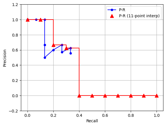
Figure 4: Demo P-R curve. Blue curve is the computed P-R values taken from Table 1 (assuming N = 15). Red curve is the 11-point interpolated curve.
Below is the Python code to generate Figure 4:
import numpy as np
import matplotlib.pyplot as plt

tp = np.array([1, 1, 0, 0, 1, 1, 0, 1, 0]) # true positive flags
fp = 1 - tp                                # false positive flags
acc_tp = np.cumsum(tp)                     # accumulative sum
acc_fp = np.cumsum(fp)

N = 15                                     # total number of labels
pre = acc_tp / (acc_tp + acc_fp)           # precision
rec = acc_tp / N                           # recall

pre = np.r_[1., pre]                       # add a beginning point
rec = np.r_[0., rec]

# do 11-point interpolation
rec_interp = np.linspace(0, 1, 11, endpoint=True)
pre_interp = []
for rii in rec_interp:
    p_on_right = pre[rec>=rii]
    if len(p_on_right) > 0:
        pii = np.max(p_on_right)
    else:
        pii = 0
    pre_interp.append(pii)

#-------------------Plot------------------------
figure = plt.figure()
ax = figure.add_subplot(1,1,1)

ax.plot(rec, pre, 'b-o', ms=5, label='P-R')
ax.step(rec_interp, pre_interp, where='post', color='r')
ax.plot(rec_interp, pre_interp, marker='^', ms=8, ls='none', color='r', label='P-R (11-point interp)')
ax.set_xlabel('Recall')
ax.set_ylabel('Precision')
ax.set_ylim(-0.2, 1.2)
ax.grid(True, axis='both')
ax.legend()
figure.show()
4.4. Python code for AP computation
Code first:
def compute_AP(pred, label, class_idx, conf_thres=0.25, iou_thres=0.5, interp=11):
    '''Compute Average Precision for a class

    Args:
        pred (ndarray): predictions, in shape (n, 7). n is the number of detections.
            The columns are: [batch_idx, x_c, y_c, w, h, conf, clss].
        label (ndarray): ground truth labels, in shape (m, 6). m is the number
            of labels. The columns are: [batch_idx, x_c, y_c, w, h, clss].
        class_idx (int): target class idx.
    Keyword Args:
        conf_thres (float): optionally filter prediction by confidence score.
        iou_thres (float): IoU score threshold to flag true/false positives.
        interp (int or None): if None, compute Area Under Curve using trapz
            integration. If 11, smooth the P-R curve using 11-point interpolation.
    Returns:
        precision (ndarray): 1d array, precision values.
        recall (ndarray): 1d array, recall values.
        ap (float): average precision.
    '''

    # select class
    pred = pred[pred[:, -1] == class_idx]
    label = label[label[:, -1] == class_idx]

    if len(pred) == 0:
        return 0, 0, 0

    # filter by confidence
    conf_idx = np.where(pred[:, 5] >= conf_thres)[0]
    if len(conf_idx) == 0:
        # all false positive
        return 0, 0, 0

    npred = len(pred)
    nlabel = len(label)
    tp = np.zeros(npred, dtype='int')   # true positive flags
    label_visited = np.zeros(nlabel, dtype='int')  # record labels that have been matched with a detection

    # loop through detections
    for idxii in conf_idx:
        pii = pred[[idxii]]

        # select labels in same image
        labidx = np.where(label[:, 0] == pii[:, 0])[0]
        labii = label[labidx]
        if len(labii) == 0:
            # no matching label, false positive
            continue

        # compute iou with labels
        ious = compute_IOU(pii[:, 1:5], labii[:, 1:5], x1y1x2y2=False, change_enclose=False)
        # get the  closest label
        best_iou_idx = np.argmax(ious)
        best_iou = ious[best_iou_idx]
        all_labidx = labidx[best_iou_idx]

        if best_iou >= iou_thres and label_visited[all_labidx] == 0:
            tp[idxii] = 1                  # mark this prediction true positive
            label_visited[all_labidx] = 1  # mark this label as visited

    # build the AP computing table
    # sort by conf
    conf_idx = np.argsort(pred[:, 5])[::-1]
    pred = pred[conf_idx]
    tp = tp[conf_idx]
    fp = 1 - tp
    acc_tp = np.cumsum(tp)
    acc_fp = np.cumsum(fp)

    precision = acc_tp / (acc_tp + acc_fp + 1e-6)
    recall = acc_tp / nlabel

    # add starting point
    precision = np.r_[1., precision]
    recall = np.r_[0., recall]

    # do interpolation if needed
    if not interp:
        ap = np.trapz(precision, recall)
    elif interp == 11:
        rr = np.linspace(0, 1, 11, endpoint=True)
        ap = 0
        for rii in rr:
            pre_on_right = precision[recall >= rii]
            if len(pre_on_right):
                ap += np.max(pre_on_right)
        ap /= 11
    else:
        raise Exception("<interp> is None or 11.")

    return precision, recall, ap
Some explanations:
Remember that AP is class-specific, so we start by selecting the correct class. If nothing gets selected, then true positive detections, precision and AP are all 0:
# select class
pred = pred[pred[:, -1] == class_idx]
label = label[label[:, -1] == class_idx]

if len(pred) == 0:
    return 0, 0, 0
We initialize an 0-valued label_visited array to record the
“visited” labels. This is because if a ground truth label is assigned
to a prediction (by having the highest IoU score among all labels), it
can not be assigned to a second prediction in the future, to avoid
double counting.
So, when we flag a prediction as true positive, we also flag that matched label as “visited”:
# compute iou with labels
ious = compute_IOU(pii[:, 1:5], labii[:, 1:5], x1y1x2y2=False, change_enclose=False)
# get the  closest label
best_iou_idx = np.argmax(ious)
best_iou = ious[best_iou_idx]
all_labidx = labidx[best_iou_idx]

if best_iou >= iou_thres and label_visited[all_labidx] == 0:
    tp[idxii] = 1                  # mark this prediction true positive
    label_visited[all_labidx] = 1  # mark this label as visited
Also note that when calling compute_IOU(), we set the
change_enclose flag to False. Because this is a different context than
NMS filtering, and we do need a lower IOU score to properly reflect
the poor matches in such enclosed cases.
4.5. Python code for mAP computation
Having got the AP computation code, it is trivial to get mAP: we simply loop through all classes to get an average:
def compute_mAP(pred, label, conf_thres=0.25, iou_thres=0.5, interp=11):
    '''Compute mean Average Precision across classes

    Args:
        pred (ndarray): predictions, in shape (n, 7). n is the number of detections.
            The columns are: [batch_idx, x_c, y_c, w, h, conf, clss].
        label (ndarray): ground truth labels, in shape (m, 6). m is the number
            of labels. The columns are: [batch_idx, x_c, y_c, w, h, clss].
    Keyword Args:
        conf_thres (float): optionally filter prediction by confidence score.
        iou_thres (float): IoU score threshold to flag true/false positives.
        interp (int or None): if None, compute Area Under Curve using trapz
            integration. If 11, smooth the P-R curve using 11-point interpolation.
    Returns:
        mAP (float): mean Average Precision.
    '''

    class_idx = np.unique(label[:, -1])
    class_aps = []
    # loop through classes
    for clsii in class_idx:
        _, _, apii = compute_AP(pred, label, clsii, conf_thres, iou_thres, interp)
        class_aps.append(apii)

    mAP = np.mean(class_aps)

    return mAP
4.6. Multiple IoU thresholds
Now it is the correct point to extend into multiple IoU threshold values.
Having got the mAP using IoU=0.5, we can iterate through the IoU range of
[0.5, 0.95], with a step of 0.05. The average mAP across these 10
IoU levels is called mAP@[0.5:0.05:0.95]. Or, using the COCO naming
convention, AP@[0.5:0.05:0.95]: they treat AP and mAP as
synonyms (thanks COCO for the confusion).
5. Summary
In this post we create 3 essential tools in object detection task:
- Intersection-Over-Union (IoU): a goodness of match metric between a bounding box prediction and a ground truth label.
- Non-Maximum suppression (NMS): a method to filter out duplicate detections.
- mean Average Precision (mAP): a metric of the overall accuracy of a detection model.
All these will be used in later posts when we write the model-training
code, and it is a good idea to store these functions in the utils.py
script in the YOLOv3_pytorch project folder.
Created: 2022-06-22 Wed 22:40


