Table of Contents
1. Overview
This is Part-5 of the series on building a YOLOv3 model from scratch.
Here is an overview of the series:
- Understand the YOLO model.
- Build the model backbone.
- Load pre-trained weights.
- Get the tools ready.
Training data preparation: this post.
This part will write some pre-processing codes to load the COCO detection dataset, including the images and annotation labels. It is also a good chance to test out the IoU, NMS and mAP utility functions we created in the last part.
- Train the model.
2. Get the COCO data
I used this bash script from the Github repo of darknet to download the 2014 COCO detection dataset.
It is generally a good practice to examine the bash script before executing it. So download the script file, have a look, put it somewhere and execute it. It will download the 2014 COCO training and validation datasets, as well labels. The entire unzipped dataset is about 23 GB in size, so make sure your disk has enough of space.
Once it is done, we should have a folder structure like this:
coco/
   images/
       train2014/
       val2014/
   labels/
       train2014/
       val2014/
   ...
I’ve omitted other files and folders. We will be focusing on the
images and labels folders alone.
It might be a good idea to symlink this coco folder into the data
sub-folder under the YOLOv3_pytorch project folder. For a structure
of the folder, refer back to the Create the Darknet-53 model section
of part-2.
Also note that we will need to map the class names to ids and back. So
also put this coco.names_.txt file into the coco folder as well.
3. Create dataset and dataloader objects
I’m going to put the relevant code in a loader.py script in the
YOLOv3_pytorch project folder. You can put these anywhere you like.
3.1. The COCODataset class
Here is the definition of the COCODataset class:
class COCODataset(Dataset):
    '''Create Dataset for COCO data

    Args:
        base_folder (str): base folder for the coco data. Should contain sub-folders
            of "images" and "labels".
    Keyword Args:
        train (bool): if True, load training data. Otherwise load valication data.
        transform (torchvision.transforms or None): transform to perform on loaded images.
            If None, will do a ToTensor() transform by default.
        max_size (int or None): if not None, select only the first <max_size> samples.
    '''
    def __init__(self, base_folder, train=True, transform=None, max_size=None):
        Dataset.__init__(self)

        self.base_folder = base_folder
        self.train = train

        if transform is not None:
            self.transform = transform
        else:
            self.transform = transforms.ToTensor()

        # class2id and id2class dicts
        self.cls_name_file = os.path.join(base_folder, 'coco.names_.txt')
        self.class2id, self.id2class = read_coco_names(self.cls_name_file)

        if train:
            self.image_folder = os.path.join(base_folder, 'images', 'train2014')
            self.label_folder = os.path.join(base_folder, 'labels', 'train2014')
        else:
            self.image_folder = os.path.join(base_folder, 'images', 'val2014')
            self.label_folder = os.path.join(base_folder, 'labels', 'val2014')

        self.image_files = os.listdir(self.image_folder)
        self.label_files = os.listdir(self.label_folder)
        self.image_files.sort()
        self.label_files.sort()

        if max_size is not None:
            self.image_files = self.image_files[:max_size]
            self.label_files = self.label_files[:max_size]

        self.image_files = [os.path.join(self.image_folder, ii) for ii in self.image_files]
        self.label_files = [os.path.join(self.label_folder, ii) for ii in self.label_files]

    def __len__(self):
        return len(self.image_files)

    def __getitem__(self, idx):

        idx = idx % len(self.image_files)

        # get image
        image_file = self.image_files[idx]
        image = Image.open(image_file).convert('RGB')
        image = self.transform(image)

        # prepare label
        label_file = self.label_files[idx]
        labels = np.loadtxt(label_file)  # cls, x, y, w, h
        labels = np.atleast_2d(labels)
        labels = np.roll(labels, -1, axis=1)  # x, y, w, h, cls

        labels = torch.from_numpy(labels).float()

        return image, labels
Some points to note:
- If the input argument
trainisTrue, we load the training data fromcoco/images/train2014. Otherwise, we load validation data fromcoco/images/val2014. - The input
transformargument can be used to do data augmentation. Just be careful that the transformations should be label-preserving. Remember, we are dealing with bounding box coordinates, so make sure the labels are changed in a consistent way. - We add an optional
max_sizeargument to select only a subset of the dataset. This could be helpful when doing small trials to make sure that the model is capable of overfitting a small dataset. For each image file, e.g.
coco/images/train2014/COCO_train2014_000000000089.jpg, there is a corresponding label file, e.g.coco/labels/train2014/COCO_train2014_000000000089.txtThe content of the label file looks like this:43 0.805492 0.357625 0.040359 0.275792 43 0.760125 0.376135 0.030812 0.221062 43 0.846930 0.350510 0.041359 0.287271 43 0.884539 0.354979 0.032609 0.289542 43 0.917523 0.349990 0.042141 0.297479 69 0.478883 0.703823 0.525328 0.563062 68 0.092344 0.241927 0.184688 0.301896 73 0.815477 0.727354 0.141328 0.063250 73 0.865914 0.795917 0.178203 0.070208 73 0.900883 0.891187 0.198234 0.104417The 5 columns are:
- class index, from 0 to 79.
- xcenter of bounding box.
- ycenter of bounding box.
- width of bounding box.
- height of bounding box.
All coordinates are fractional offsets with respect to the top-left corner of the image, and width/height sizes are fractions of the image size.
When outputting the label, we change the columns to a layout of: [xcenter, ycenter, w, h, cls]. This is done using these 2 lines:
  labels = np.atleast_2d(labels)
  labels = np.roll(labels, -1, axis=1)  # x, y, w, h, cls
3.2. The dataloader object
I created a create_loader() function to return an instance of
COCODataset, and an instance of DataLoader:
def create_loader(data_folder, config, shuffle=True):
    '''Create a Dataset and a DataLoader obj

    Args:
        data_folder (str): base folder of the coco dataset.
        config (dict): config dict. Loaded from config/load_config.py
    Keyword Args:
        shuffle (bool): whether to shuffle the batch in DataLoader.
    Returns:
        dataset (torch.utils.data.Dataset): coco dataset.
        dataloader (torch.utils.data.DataLoader): dataloader obj.
    '''

    is_train = config['is_train']
    max_data_size = config['max_data_size']
    batch_size = config['batch_size']

    trans = transforms.Compose([
        transforms.Resize([config['width'], config['height']]),
        transforms.ToTensor()])

    dataset = COCODataset(data_folder, is_train, trans, max_data_size)
    dataloader = DataLoader(dataset, shuffle=shuffle, batch_size=batch_size,
            collate_fn=collate_fn)

    return dataset, dataloader
The input argument config is a dict containing some model parameters.
We also need a collate_fn function to pass to the DataLoader
initializer. This is because the number of objects in different
images are not the same, and DataLoader needs a way to properly
handle non-uniform sizes when preparing a batch. Besides, we also need
to label the images in a batch with indices, to keep track of which
predictions are for which images.
Here is the collate_fn() function:
def collate_fn(batch):

    samples = []
    targets = []
    for ii, (sii, tii) in enumerate(batch):
        samples.append(sii) # image

        # add batch idx to label
        tii = torch.cat([torch.full([len(tii), 1], ii).float(), tii], dim=1)
        targets.append(tii)

    samples = torch.stack(samples, 0)
    targets = torch.cat(targets, 0)

    return samples, targets
Note that after passing through the collate_fn, the labels have 6
columns:
[batch_idx, x_center, y_center, w, h, cls]
4. Test drive
Let’s test out the above shown codes. It might be a good place to also test out the codes of IoU, NMS and mAP computations, introduced in the previous part.
Create a new evaluate.py script in the YOLOv3_pytorch project
folder, with the following content:
import numpy as np
import torch
from torchvision import transforms

from config import load_config
from model import Darknet53
from utils import batch_NMS, compute_mAP, draw_predictions
from loader import create_loader

if __name__=='__main__':

    #--------------------Load model config--------------------
    CONFIG_FILE = './config/yolov3.cfg'
    net_config, module_list = load_config.parse_config(CONFIG_FILE)
    config = {'net': net_config}
    config['module_list'] = module_list
    config['width'] = 416
    config['height'] = 416
    config['n_classes'] = 80
    config['max_data_size'] = 10
    config['batch_size'] = 4
    config['is_train'] = False
    config['conf_thres'] = 0.3
    config['nms_iou_thres'] = 0.5
    config['map_iou_thres'] = 0.5
    DATA_FOLDER = './data/coco'
    WEIGHT_PATH = './yolov3.weights'

    #-------------------Create model-------------------
    model = Darknet53(config)

    #-------------------Load weights-------------------
    model.load_weights(WEIGHT_PATH)

    #----------------Turn on eval model----------------
    model.eval()

    #--------------Get dataset and dataloader--------------
    dataset, dataloader = create_loader(DATA_FOLDER, config, shuffle=False)
    id2class = dataset.id2class

    #-----------------Start prediction-----------------
    preds = []
    labels = []

    for imgii, labelii in dataloader:

        with torch.no_grad():
            yii = model(imgii)

        labelii = labelii.cpu().numpy()
        yii = yii.detach().cpu().numpy()

        # filter by NMS
        yii = batch_NMS(yii, config['conf_thres'], config['nms_iou_thres'])

        # convert to fractional coordinates and sizes, to match with labels
        yii[:, [1,3]] /= config['width']
        yii[:, [2,4]] /= config['height']

        print('## yii.shape:', yii.shape)
        print('## labelii.shape:', labelii.shape)
        preds.append(yii)
        labels.append(labelii)

        # draw predictions
        if len(yii) > 0:
            # loop through images in batch
            for jj in range(len(imgii)):
                imgjj = imgii[jj]           # get image from batch
                imgjj = transforms.ToPILImage()(imgjj)   # transform image to PIL image
                yjj = yii[yii[:, 0] == jj][:, 1:]        # get predictions from batch
                yjj[:, [0, 2]] *= config['width']        # scale back to pixel units
                yjj[:, [1, 3]] *= config['height']

                fig, ax = draw_predictions(imgjj, model.width, model.height, yjj, id2class)
                #fig.show()

                #----------------- Save plot------------
                plot_save_name = 'pred_result_%d-%d' %(len(preds), jj)
                print('\n# <predict_pretrained>: Save figure to', plot_save_name)
                fig.savefig(plot_save_name, dpi=100, bbox_inches='tight')

    preds = np.vstack(preds)
    labels = np.vstack(labels)
    print(preds.shape)
    print(labels.shape)

    mAP = compute_mAP(preds, labels, 0, config['map_iou_thres'])
    print('mAP@0.5 =', mAP)
Some points to note:
We use many building blocks created in earlier parts:
from config import load_config
from model import Darknet53
from utils import batch_NMS, compute_mAP, draw_predictions
So if you haven’t got these ready, please go back to previous parts of the series first.
We call the newly created
create_loader()function to get thedatasetanddataloader. For test purposes, I’m reading in only 10 images, with a batch size of 4:config['max_data_size'] = 10 config['batch_size'] = 4
- When iterating through the
dataloader,imgiiis a 4D tensor with shape[B, 3, 416, 416], whereBis the batch size.labeliiis a 2D tensor of shape[n, 6], wherenis the number of labeled objects in this batch. There are some back-n-forth coordinate transformations.
  yii[:, [1,3]] /= config['width']
  yii[:, [2,4]] /= config['height']
This is converting the model predicted bounding box coordinates to fractional units, because the labels are using fractions, and we need them to be consistent to compute the mAP.
When creating the plot using
draw_predictions(), we convert from fractions back to pixel units again:imgjj = transforms.ToPILImage()(imgjj) # transform image to PIL image yjj = yii[yii[:, 0] == jj][:, 1:] # get predictions from batch yjj[:, [0, 2]] *= config['width'] # scale back to pixel units yjj[:, [1, 3]] *= config['height']
- To compute the mAP score, we collect all predictions in the
predslist, and all labels in thelabelslist, convert them tonp.ndarray, and call ourcompute_mAP()function created in the previous post.
Below are some sample image outputs. Note that the NMS process has eliminated duplicate predictions. But when there are many objects relatively packed together, they are also all preserved.
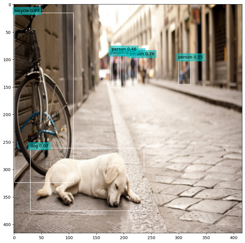
Figure 1: Sample image with detection results.
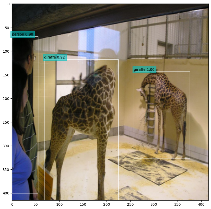
Figure 2: Sample image with detection results.
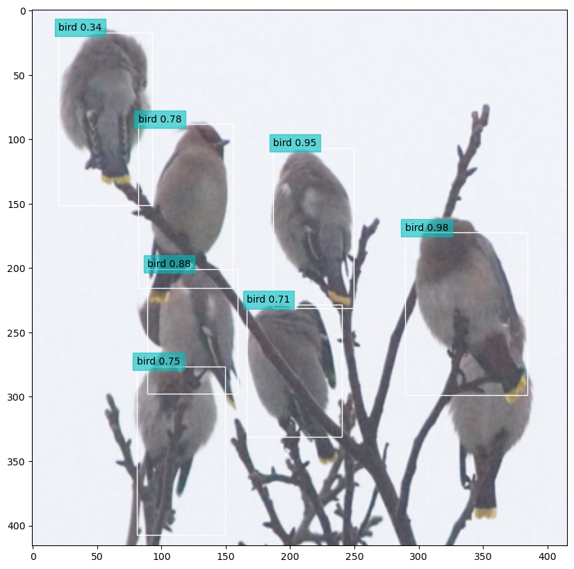
Figure 3: Sample image with detection results.
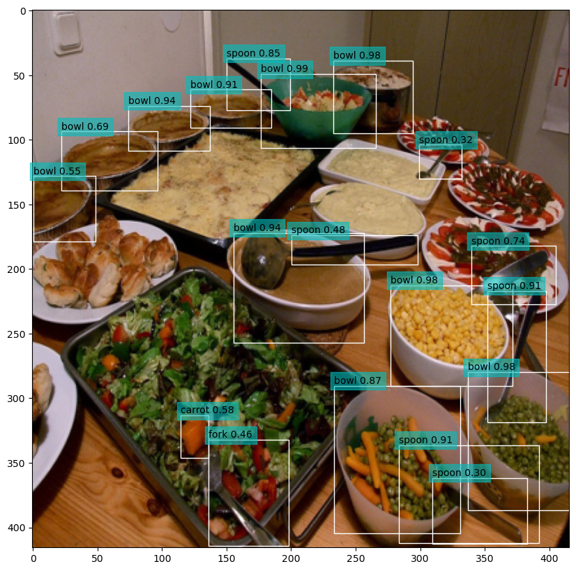
Figure 4: Sample image with detection results.
The final mAP@0.5 score is 0.53. The validation sample size is too
small (we only used 10 images) for this to be really meaningful, but
it is comparable with the reported offical value.
5. Summary
In this post we created Dataset and DataLoader classes to
read and load COCO 2014 detection data, then tested out the IoU,
NMS and mAP computation functions.
We have got everything ready to start training a YOLOv3 model from scratch, or do some fine-tuning with pre-trained weights. We will get into the training part in the next post.
Created: 2022-06-22 Wed 22:42


