Table of Contents
1. Overview
This is Part-6 of the series on building a YOLOv3 model from scratch.
Here is an overview of the series:
- Understand the YOLO model.
- Build the model backbone.
- Load pre-trained weights.
- Get the tools ready.
- Training data preparation.
Train the model: This post.
Whether to perform fine-tuning, or train a new model on a different type of data from scratch, we need to have properly working training codes.
1.1. Plan of this post
We already implemented the prediction functionality in Part-2, and tested it out using pre-trained weights in Part-3.
The training part is, in my opinion, considerably more complex in comparison. I guess this is partly because the inference code is all predicated on what the model is “supposed” to work, and we all know that it does work. But for the training part, we need to figure out a “how”: “how” do we make the model learn to work the way it is “supposed” to work.
Another reason that training code is more difficult to develop is simply that it takes a much longer time to do the computations, and you will have to monitor the convergence of the model, if it ever converges at all. And for a model like YOLO, it does impose some hardware requirement. A gaming laptop/desktop equipped with a GPU will do much better than a CPU-only setup.
For illustration purposes, I’m going to train from scratch on only a tiny sub-set of the COCO dataset.
This is we are going to achieve in this post:
- Write a new
train.pyscript, in which: - Instantiate a YOLOv3 model.
- Load a sub-set of the COCO 2014 detection data.
- Write the training iterations, print and visualize the loss function evolution.
- Compare 3 slightly different ways to formulate the loss function.
This last point is because I’ve seen different ways to formulate the loss function in 3rd party PyTorch implementations than in the YOLO papers. I’d like to do some experiments, and share my own understandings about the results.
1.2. Some prerequisites
- All previous parts of the series.
- A machine with PyTorch installed. The beefier the better. A GPU is much preferred.
- The
tensorboardpackage, used to monitor the training process. In the simplest case, it can be installed usingpip install tensorboard.
2. Loss function of YOLO
Because YOLO is a multi-task model that predicts localization as well as classification, its loss function is also a multi-part one:
- loss term for the localization task: labeled as
loss_box. - loss term for the classification task: labeled as
loss_cls. - loss term for the objectness prediction task: labeled as
loss_obj.
loss_obj penalizes wrong predictions about the existence of
objects, either by missing an object when there is one, or predicting an
object when there is none.
2.1. YOLOv1 loss function
Below is the YOLOv1 loss function definition given in the YOLOv1 paper:
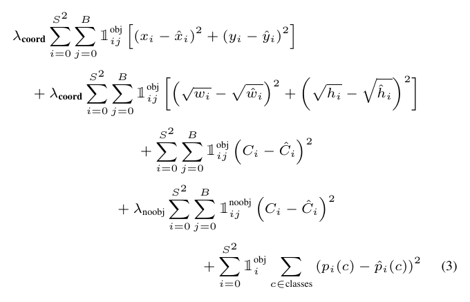
Figure 1: Loss function of YOLOv1.
where:
- \([(x_i – \hat{x_i})^2 + (y_i – \hat{y_i})^2]\): the MSE loss for bounding box location predictions.
- \([(\sqrt{w_i} – \sqrt{\hat{w_i}})^2 + (\sqrt{h_i} – \sqrt{\hat{h_i}})^2]\): the MSE loss for the bounding box size predictions. Taking the square-root on width/height is because the same amount of size errors matters differently for a large bounding box and a small one. The author used this simple method to reduce this size dependence.
- \(\mathbb{1}_{ij}^{obj} (C_i – \hat{C_i})^2\): (on 3rd row) is the loss term associated with objectness scores, when there is a ground truth object. I.e. it penalizes false negative object detections.
- \(\mathbb{1}_{ij}^{noobj} (C_i – \hat{C_i})^2\): (on 4th row) is the loss term associated with objectness scores, when there is no ground truth object. I.e. it penalizes false positive object detections.
- \(\sum_{c \in classes} (p_i(c) – \hat{p_i}(c))^2\): the MSE loss for classification predictions.
- \(\sum_{i=0}^{S^2}\): is iterating through all the cells in a feature map. Recall that for YOLOv1 on VOC data, they used \(S=7\).
- \(\sum_{j=0}^B\): is iterating through the bounding boxes in each cell. Recall that for YOLOv1 on VOC data, they used \(B=2\).
- \(\mathbb{1}_{i}\) denotes the appearance of an object in cell \(i\).
- \(\mathbb{1}_{ij}\) denotes the appearance of an object in cell \(i\), and that is associated with the jth bounding box.
- \(\lambda_{coord}\): a scaling factor to adjust the relative importance of coordinate prediction errors.
- \(\lambda_{noobj}\): a scaling factor to counter the imbalance between ground truth labels and total number of object detections.
2.2. YOLOv3 loss function
It is important to keep in mind that this is the design in YOLOv1, and some parts have been changed in YOLOv3:
- Each cell can predict different classes: this is mentioned also in Part-1, that since YOLOv2, detections in each predicting cell can be of different classes. Therefore, the term on the last line of Eq 1 is changed to
\[ \sum_{i=0}^{S^2} \sum_{j=0}^{B} \mathbb{1}_{ij}^{obj} \sum_{c \in classes} BCE(p_i(c), \hat{p_i}(c)) \]
Classification loss is changed from MSE to Binary Cross-Entropy (BCE):
  We do not use a softmax as we have found it is unnecessary for
  good performance, instead we simply use independent logistic
  classifiers. Dur- ing training we use binary cross-entropy loss
  for the class predictions.
[from YOLOv3 paper]
This is also reflected in the equation above.
2.3. The \(\mathbb{1}\) (\mathbb{1}) term
In my opinion, the \(\mathbb{1}\) term (for some reason \mathbb{1} is
not typeset correctly in HTML export) is of crucial importance, and
might not be obvious how to compute exactly. Here are some
descriptions about this term in YOLOv1 paper:
where \(\mathbb{1}_i^{obj}\) denotes if object appears in cell \(i\) and \(\mathbb{1}_i^{obj}\) denotes that the $j$th bounding box predictor in cell \(i\) is “responsible” for that prediction.
YOLO predicts multiple bounding boxes per grid cell. At training time we only want one bounding box predictor to be responsible for each object. We assign one predictor to be “responsible” for predicting an object based on which prediction has the highest current IOU with the ground truth. This leads to specialization between the bounding box predictors. Each predictor gets better at predicting certain sizes, aspect ratios, or classes of object, improving overall recall.
It also only penalizes bounding box coordinate error if that predictor is “responsible” for the ground truth box (i.e. has the highest IOU of any predictor in that grid cell).
In the YOLOv3 paper:
our system only assigns one bounding box prior for each ground truth object. If a bounding box prior is not assigned to a ground truth object it incurs no loss for coordinate or class predictions, only objectness.
From these descriptions, we know that \(\mathbb{1}\) describes some kind of “exclusive” association between a ground truth object, and one of the anchor boxes, in that same cell as the ground truth object. This chosen anchor box is then regarded as “responsible” for predicting that object, therefore any loss incurred during the process will be assigned to that anchor box.
So, for any ground truth object, determining \(\mathbb{1}_{ij}^{obj}\) amounts to determining 3 numbers, at least:
- \(i\), \(j\): indices of the predicting cell in a feature map.
- \(a\): index of the anchor box prior in the cell of \((i,j)\).
To find \((i,j)\), we only need to work out the center location of the ground truth object, measured in feature coordinate (refer back to Part-1).
To find \(a\), the paper described it as finding the anchor that “has the highest IOU of any predictor in that grid cell”.
Having got the triplet \((i,j,a)\), we can pin-point a specific anchor box in a specific cell, to address any loss during the prediction process.
But, there are a couple of more things to consider:
- YOLOv3 predicts at 3 scales: large scale, mid scale and small scale. Let’s label this scale dimension coordinate \(s\). So we have a 4th coordinate to pin-point that “responsible” anchor box: \((s,i,j,a)\).
- In each training iteration, usually multiple images are read to form a batch. Suppose \(B\) images are loaded in a batch, so they are given indices \(b=\{0, 1, \cdots, B-1\}\). Corresponding to these images there are \(N\) ground truth labels, indexed \(n = \{0, 1, \cdots, n-1\}\). Therefore, when assigning a responsible anchor for each label, we also need to keep track of \(b\) and \(n\).
To summarize: \(\mathbb{1}\) amounts to building the correct indices that associate the ground truth labels with responsible anchor boxes. Practically, we need these 6 coordinates:
\[(s, n, b, a, i, j)\]
where:
- \(s\): scale index, 0, 1, or 2.
- \(n\): label index, 0 to \(N-1\).
- \(b\): batch index, 0 to \(B-1\).
- \(a\): anchor box index, 0, 1, or 2.
- \(i, j\): feature map cell location indices. Depends on \(s\).
When implementing in PyTorch, I tried 2 different ways of building these indices. More details are given later.
2.4. Localization loss: MSE v.s. 1 – IoU
In the YOLO papers, localization loss consists of 2 MSE losses for the x, y locations, and for the width, height sizes (see Eq 1).
When reading other people’s implementation, I found another formulation of the localization loss: 1 – IoU.
This makes sense, since the final metric, mAP, is heavily predicated on IoU. Interestingly, 1 – IoU was already used as a distance metric when performing K-Means clustering to determine the anchor box priors (see YOLOv2 paper).
So, there are at least 2 ways to formulate the loss_box term: MSE
and 1 – IoU. I did some simple experiments comparing
the two. The results are given later.
2.5. Objectness target: 1 v.s. IoU
This part is more of my own understanding, or rather, misunderstanding about the objectness prediction.
It is stated in the YOLOv1 paper that:
These confidence scores reflect how confident the model is that the box contains an object and also how accurate it thinks the box is that it predicts. Formally we define confidence as Pr(Object) ∗ \(IOU_{pred}^{truth}\). If no object exists in that cell, the confidence scores should be zero. Otherwise we want the confidence score to equal the intersection over union (IOU) between the predicted box and the ground truth.
And in the YOLOv2 paper:
Following YOLO, the objectness prediction still predicts the IOU of the ground truth and the proposed box.
So it was made quite clear that the target value of objectness prediction is the IoU score.
But, not sure about you, my intuitive response was: shouldn’t the objectness target of ground truth label be 1?
So I tested it out, by comparing 2 ways of formulating the loss_obj
term: using 1.0 as target value, and using IoU as the target
values. The results are given later, but the conclusion
is: the IoU target works better.
3. PyTorch implementation
3.1. Quick recap
Let’s do a quick recap on the format of model outputs and target labels.
We have the following snippet in the training iteration:
for ii, (imgii, labelii) in enumerate(dataloader):
    model.train()
    imgii = imgii.to(device)
    labelii = labelii.to(device)
    yhatii = model(imgii)
    lossii = compute_loss(yhatii, labelii, model)
    lossii.backward()
Where:
imgiiis a 4D tensor, with shape[batch_size, 3, 416, 416].labeliiis a 2D tensor, with shape[n_labels, 6]. The 6 columns are:[batch_idx, x_center, y_center, w, h, cls]
yhatiiis the model output in training mode. It is alistof 3 tensors, corresponding to predictions at 3 size scales. Each tensor has a shape of[batch_size, n_anchors, h, w, 5 + n_classes].
More details about these are given in Part-2, Build the model backbone, and Part-5, Training data preparation.
3.2. The compute_loss() function
Code first:
def compute_loss(yhat, label, model, bbox_loss='iou', obj_label='1'):
    '''Compute multi-task losses

    Args:
        yhat (list of tensors): YOLO model output at 3 scales in a list. Each
            tensor has shape [B, na, h, w, 5 + n_classes]. Where:
            B: batch_size. na: number of anchors.
            h: number of rows. w: number of columns.
            Columns of last dimension: [x_center, y_center, w, h, obj, c1, ..., ck].
        label (tensor): ground truth label, in shape (n, 6). n: number of labeled
            objects in the batch. Columns: [batch_idx, x_center, y_center, w, h, cls].
        model (nn.Module): YOLO model.
    Keyword Args:
        bbox_loss (str): 'mse': use MSE loss for the x,y centers and w,h sizes.
            'iou': use IoU with label bbox as loss.
        obj_label (str): '1': use 1 as the target objectness score in label
            locations. 'iou': use IoU between prediction and ground truth as
            target objectness score in label locations.
    Returns:
        loss_box (nn.Variable): loss term from bounding box prediction.
        loss_obj (nn.Variable): loss term from objectness score prediction.
        loss_cls (nn.Variable): loss term from classification prediction.
    '''

    n_class = model.n_classes
    device = label.device

    # compute a factor to counter unbalanced object labels
    n_labels = len(label)   # num of objects in label
    n_preds = 0             # total num of predictions
    for yhatii in yhat:
        b, na, h, w, _ = yhatii.shape
        n_preds += na * h * w

    obj_weights = torch.tensor([(n_preds - n_labels)/n_labels*0.5]).to(device)

    # prepare loss terms
    loss_box = torch.zeros(1, device=device)
    loss_obj = torch.zeros(1, device=device)
    loss_cls = torch.zeros(1, device=device)
    if bbox_loss == 'mse':
        loss_xy = torch.zeros(1, device=device)
        loss_wh = torch.zeros(1, device=device)

    # BCE loss func for objectness score and classification
    obj_bce = nn.BCEWithLogitsLoss(pos_weight=obj_weights)
    cls_bce = nn.BCEWithLogitsLoss()

    if bbox_loss == 'mse':
        # MSE loss func for x,y,w,h
        xy_mse = nn.MSELoss()
        wh_mse = nn.MSELoss()

    # loop through 3 scales
    for yhatii, yoloii in zip(yhat, model.yolo_layers):

        b, na, h, w, _ = yhatii.shape
        stride = float(yoloii.stride)
        anchors = (yoloii.anchors / stride).float().to(device) # [n_anchors, 2]
        grid_size = torch.tensor([w, h]).float().to(device)

        # w, h from labels, convert to feature map scale
        wh_lb = label[:, 3:5] * grid_size  # [n_label, 2]

        # find matches between labels and anchors
        ratio = wh_lb[:, None, :] / anchors[None, :, :]  # [n_label, n_anchors, 2]
        ratio = torch.abs(ratio - 1).sum(2)  # [n_label, n_anchors]
        # select anchor boxes with closest ratios
        ratio = torch.min(ratio, dim=1)
        # labeled object index
        label_idx = ratio[0] < 2     # 2 is empirical
        # anchor index
        anchor_idx = ratio[1][label_idx]

        # get batch indices of labeled objects
        batch_idx = label[label_idx, 0].long()

        # get cell indices of labeled objects
        xy_lb = label[label_idx, 1:3] * grid_size
        xy_idx = torch.floor(xy_lb).long()
        x_idx = xy_idx[:,0].clamp(0, int(grid_size[0])-1)
        y_idx = xy_idx[:,1].clamp(0, int(grid_size[1])-1)

        # get target objectness scores
        obj_lb = torch.zeros(yhatii.shape[:-1]).float().to(device=device)
        if obj_label == '1':
            obj_lb[batch_idx, anchor_idx, y_idx, x_idx] = 1

        # predicted objectness scores
        obj_pd = yhatii[..., 4]

        # if there are target objects in this scale:
        if len(batch_idx) > 0:
            # relative offsets wrt to cells of labels
            relxy_lb = xy_lb - xy_idx

            # x,y offests of predictions
            xy_pd = torch.sigmoid(yhatii[batch_idx, anchor_idx, y_idx, x_idx, 0:2])

            # w,h sizes of labels
            wh_lb = label[label_idx, 3:5] * grid_size

            # w,h sizes of predictions, in feature map coordinate
            wh_pd = torch.exp(yhatii[batch_idx, anchor_idx, y_idx, x_idx, 2:4]) * anchors[anchor_idx, :]
            wh_pd = wh_pd.clamp(0, grid_size.max())

            if bbox_loss == 'mse':
                # x,y mse loss
                loss_xy += xy_mse(xy_pd, relxy_lb)
                # w,h mse loss
                loss_wh += wh_mse(wh_pd, wh_lb) / 10   # scale size loss down
                loss_box += (loss_xy + loss_wh)

            if bbox_loss == 'iou' or obj_label == 'iou':
                # compute IoUs
                pbox = torch.cat([xy_pd, wh_pd], dim=1)
                box_lb = torch.cat([relxy_lb, wh_lb], dim=1)
                iou = compute_IOU(pbox, box_lb, x1y1x2y2=False, change_enclose=False)
                loss_box += (1.0 - iou).mean()

                if obj_label == 'iou':
                    # Use cells with iou > 0 as object targets
                    obj_lb[batch_idx, anchor_idx, y_idx, x_idx] = iou.detach().clamp(0).type(obj_lb.dtype)
            # classification predictions
            cls_pd = yhatii[batch_idx, anchor_idx, y_idx, x_idx, 5:]

            # one-hot encode classes
            cls_one_hot_lb = F.one_hot(label[label_idx, -1].long(), n_class).float().to(device)
            # classification loss
            loss_cls += cls_bce(cls_pd, cls_one_hot_lb)

        # objectness score loss
        loss_obj += obj_bce(obj_pd, obj_lb)

    loss = loss_box + loss_obj + loss_cls

    return loss, loss_box , loss_obj , loss_cls
More explanations:
The
bbox_lossinput argument has 2 choices:'mse'or'iou'. These are the 2 ways of formulating the localization loss mentioned above. I added this only for experiment purposes.If this is set to
'mse', anMSELoss()loss function is created for the x, y coordinates, and another one for the w, h sizes:if bbox_loss == 'mse': # MSE loss func for x,y,w,h xy_mse = nn.MSELoss() wh_mse = nn.MSELoss()
Later, the
loss_boxterm is computed as the sum of the 2:if bbox_loss == 'mse': # x,y mse loss loss_xy += xy_mse(xy_pd, relxy_lb) # w,h mse loss loss_wh += wh_mse(wh_pd, wh_lb) / 10 # scale size loss down loss_box += (loss_xy + loss_wh)
If
bbox_lossis set to'iou',loss_boxis computed using:if bbox_loss == 'iou' or obj_label == 'iou': # compute IoUs pbox = torch.cat([xy_pd, wh_pd], dim=1) box_lb = torch.cat([relxy_lb, wh_lb], dim=1) iou = compute_IOU(pbox, box_lb, x1y1x2y2=False, change_enclose=False) loss_box += (1.0 - iou).mean()
The
obj_labelinput argument has 2 choices'1'or'iou'. These are the 2 ways of setting the objectness target values mentioned above. Again, for test purposes only.If
obj_label == '1', set objectness target values to 1:# get target objectness scores obj_lb = torch.zeros(yhatii.shape[:-1]).float().to(device=device) if obj_label == '1': obj_lb[batch_idx, anchor_idx, y_idx, x_idx] = 1
where
batch_idx,anchor_idx,y_idx,x_idxcorrespond to the \((b, a, i, j)\) coordinates talked about earlier. More on this later.If
obj_label == 'iou', set objectness target values to IoU:if bbox_loss == 'iou' or obj_label == 'iou': # compute IoUs pbox = torch.cat([xy_pd, wh_pd], dim=1) box_lb = torch.cat([relxy_lb, wh_lb], dim=1) iou = compute_IOU(pbox, box_lb, x1y1x2y2=False, change_enclose=False) loss_box += (1.0 - iou).mean() if obj_label == 'iou': # Use cells with iou > 0 as object targets obj_lb[batch_idx, anchor_idx, y_idx, x_idx] = iou.detach().clamp(0).type(obj_lb.dtype)
I counted the number of objects/labels in the batch:
n_labels =
  len(label)
. And the total number of predictions made by the model:n_preds = 0 # total num of predictions for yhatii in yhat: b, na, h, w, _ = yhatii.shape n_preds += na * h * w
Recall that using standard settings, this is
(52 * 52 + 26 * 26 + 13 * 13) * 3 = 10647. So there would be a big imbalance between positive and negative samples. To counter this, YOLOv1 used the \(\lambda_{noobj}\) scaling factor mentioned above. I think a more specific number could actually be worked out from data:obj_weights = torch.tensor([(n_preds - n_labels)/n_labels*0.5]).to(device)
The
*0.5scaling is to tune down the ratio a bit, and it’s purely empirical.This
obj_weightsvariable works with PyTorch’sBCEWithLogitsLoss, to give weights to positive samples:# BCE loss func for objectness score and classification obj_bce = nn.BCEWithLogitsLoss(pos_weight=obj_weights)
We then loop through the 3 size scales of YOLO prediction, and get some size information first:
    # loop through 3 scales
    for yhatii, yoloii in zip(yhat, model.yolo_layers):

        b, na, h, w, _ = yhatii.shape
        stride = float(yoloii.stride)
        anchors = (yoloii.anchors / stride).float().to(device) # [n_anchors, 2]
        grid_size = torch.tensor([w, h]).float().to(device)
Note that
anchorsare convert to feature map coordinate (see Part-1), andgrid_sizeis by definition feature map sizes.The association between ground truth labels and “responsible” anchor boxes in this scale is achieved by comparing their width/height ratios:
        # w, h from labels, convert to feature map scale
        wh_lb = label[:, 3:5] * grid_size  # [n_label, 2]
        # find matches between labels and anchors
        ratio = wh_lb[:, None, :] / anchors[None, :, :]  # [n_label, n_anchors, 2]
The best matches are those with smallest absolute width+height ratios from
1.0:ratio = torch.abs(ratio - 1).sum(2) # [n_label, n_anchors] # select anchor boxes with closest ratios ratio = torch.min(ratio, dim=1) # labeled object index label_idx = ratio[0] < 2 # 2 is empirical # anchor index anchor_idx = ratio[1][label_idx]
label_idxis a tensor of indices, denoting those ground truth labels that found associations with any anchor box in this scale. This is the \(n\) coordinate mentioned in The \(\mathbb{1}\) term sub-section.anchor_idxis a tensor of indices, denoting the anchor boxes in this scale that were associated with any ground truth labels. This is the \(a\) coordinate mentioned in The \(\mathbb{1}\) term sub-section.These 2 index arrays will be used to select the relevant predictions.
To select the relevant predictions, we need these coordinates:
\[(s, n, b, a, i, j)\]
The iteration through scales implicitly gives \(s\).
We just got \(n\) and \(a\) as shown above.
\(b\) is obtained by:
        # get batch indices of labeled objects
        batch_idx = label[label_idx, 0].long()
And \(i, j\):
        # get cell indices of labeled objects
        xy_lb = label[label_idx, 1:3] * grid_size
        xy_idx = torch.floor(xy_lb).long()
        x_idx = xy_idx[:,0].clamp(0, int(grid_size[0])-1)
        y_idx = xy_idx[:,1].clamp(0, int(grid_size[1])-1)
These define the ground truth – anchor box associations.
Objectness prediction is not restricted to those “responsible” anchor boxes. Rather, all predictions are included (this is why we needed a
obj_weightsto balance the positive/negative samples):# predicted objectness scores obj_pd = yhatii[..., 4]
Labels may not be associated with anchors of a specific scale. To check this:
        # if there are target objects in this scale:
        if len(batch_idx) > 0:
            ...
The x, y location predictions are obtained using:
            # x,y offests of predictions
            xy_pd = torch.sigmoid(yhatii[batch_idx, anchor_idx, y_idx, x_idx, 0:2])
And w, h predictions:
            # w,h sizes of predictions, in feature map coordinate
            wh_pd = torch.exp(yhatii[batch_idx, anchor_idx, y_idx, x_idx, 2:4]) * \
                anchors[anchor_idx, :]
            wh_pd = wh_pd.clamp(0, grid_size.max())
Note that we use the \((b, a, i, j)\) coordinates (
[batch_idx, anchor_idx, y_idx, x_idx]) to take the correct values.Classification loss is computed by first selecting the correct values as before, and constructing one-hot encoded target values:
            # classification predictions
            cls_pd = yhatii[batch_idx, anchor_idx, y_idx, x_idx, 5:]

            # one-hot encode classes
            cls_one_hot_lb = F.one_hot(label[label_idx, -1].long(), n_class).float().to(device)
            # classification loss
            loss_cls += cls_bce(cls_pd, cls_one_hot_lb)
Note that
torch.nn.BCEWithLogitsLossexpects values without taking the sigmoid, so don’t passcls_pdto the sigmoid function, similar forobj_pd.Having gone through all 3 scales, we sum up all the loss terms and return them:
    loss = loss_box + loss_obj + loss_cls
    return loss, loss_box , loss_obj , loss_cls
3.3. An alternative compute_loss2() function
Spoiler alert: this function doesn’t work properly. So feel free to skip this.
The above compute_loss() function selects the “responsible” anchor
boxes by comparing ground truth labels with anchor box priors.
Note that in this workflow, it is possible for more than 1 anchors in different scales to be associated with a same label. I’m not sure whether this would cause any practical harm.
The compute_loss2() shown here is a closer-to-the-paper version: it
computes the IoU scores between labels and all 9 anchor boxes, and
selects the anchor with the highest IoU. This way, it is ensured that
only 1 anchor box is associated with any label.
3.3.1. select_anchor() function
To do this association, first create a select_anchor() function:
def select_anchor(yhat, label, model):

    n_labels = len(label)
    n_scales = len(yhat)
    n_anchors = yhat[0].shape[1]
    device = label.device
    batch_idx = label[:, 0].long()

    best_iou_scales = torch.zeros([n_scales, n_labels], device=device)
    best_iou_xy_pd = torch.zeros([n_scales, n_labels, n_anchors, 2], device=device)
    best_iou_wh_pd = torch.zeros([n_scales, n_labels, n_anchors, 2], device=device)
    best_iou_xy_lb = torch.zeros([n_scales, n_labels, 2], device=device)
    best_iou_wh_lb = torch.zeros([n_scales, n_labels, 2], device=device)

    best_iou_ancidx = torch.zeros([n_scales, n_labels], dtype=torch.long, device=device)
    label_x_idx = torch.zeros([n_scales, n_labels], dtype=torch.long, device=device)
    label_y_idx = torch.zeros([n_scales, n_labels], dtype=torch.long, device=device)

    # loop through 3 scales
    for ii, (yhatii, yoloii) in enumerate(zip(yhat, model.yolo_layers)):

        b, na, h, w, _ = yhatii.shape
        stride = float(yoloii.stride)
        anchors = (yoloii.anchors / stride).float().to(device) # [n_anchors, 2]
        grid_size = torch.tensor([w, h]).float().to(device)

        # get cell indices of labeled objects
        xy_lb = label[:, 1:3] * grid_size.unsqueeze(0)
        xyidx = torch.floor(xy_lb).long()
        xidx = xyidx[:,0].clamp(0, int(grid_size[0])-1)
        yidx = xyidx[:,1].clamp(0, int(grid_size[1])-1)

        # relative offsets wrt to cells of labels
        relxy_lb = xy_lb - xyidx

        # w, h from labels, convert to feature map scale
        wh_lb = label[:, 3:5] * grid_size  # [n_label, 2]

        # x,y offests of predictions
        relxy_pd = torch.sigmoid(yhatii[batch_idx, :, yidx, xidx, 0:2])

        # w,h sizes of predictions, in feature map coordinate
        wh_pd = torch.exp(yhatii[batch_idx, :, yidx, xidx, 2:4]) * anchors.unsqueeze(0)
        wh_pd = wh_pd.clamp(0, grid_size.max())

        # compute IoUs
        pbox = torch.cat([relxy_pd, wh_pd], dim=2).view([-1, 4])
        box_lb = torch.cat([relxy_lb, wh_lb], dim=1).view([-1, 1, 4])
        box_lb = box_lb.repeat(1, na, 1).view(-1, 4)
        iou = compute_IOU(pbox, box_lb, x1y1x2y2=False, change_enclose=False)
        iou = iou.view([-1, na])

        best_iou, best_ancidx = torch.max(iou, dim=1)

        best_iou_scales[ii] = best_iou
        best_iou_ancidx[ii] = best_ancidx

        best_iou_xy_pd[ii] = relxy_pd
        best_iou_wh_pd[ii] = wh_pd

        best_iou_xy_lb[ii] = relxy_lb
        best_iou_wh_lb[ii] = wh_lb

        label_x_idx[ii] = xidx
        label_y_idx[ii] = yidx

    # stack along the new scale dimension
    label_scale_idx = torch.max(best_iou_scales, dim=0)[1]
    label_anc_idx = best_iou_ancidx[label_scale_idx, torch.arange(n_labels)]
    label_y_idx = label_y_idx[label_scale_idx, torch.arange(n_labels)]
    label_x_idx = label_x_idx[label_scale_idx, torch.arange(n_labels)]

    return label_scale_idx, label_anc_idx, label_y_idx, label_x_idx, best_iou_scales,\
            best_iou_xy_pd, best_iou_wh_pd, \
            best_iou_xy_lb, best_iou_wh_lb
Some explanations:
We initialize some placeholder tensors, then go into the iteration through scales:
    best_iou_scales = torch.zeros([n_scales, n_labels], device=device)
    best_iou_xy_pd = torch.zeros([n_scales, n_labels, n_anchors, 2], device=device)
    best_iou_wh_pd = torch.zeros([n_scales, n_labels, n_anchors, 2], device=device)
    best_iou_xy_lb = torch.zeros([n_scales, n_labels, 2], device=device)
    best_iou_wh_lb = torch.zeros([n_scales, n_labels, 2], device=device)

    best_iou_ancidx = torch.zeros([n_scales, n_labels], dtype=torch.long, device=device)
    label_x_idx = torch.zeros([n_scales, n_labels], dtype=torch.long, device=device)
    label_y_idx = torch.zeros([n_scales, n_labels], dtype=torch.long, device=device)

    # loop through 3 scales
    for ii, (yhatii, yoloii) in enumerate(zip(yhat, model.yolo_layers)):
        ...
We construct bounding boxes from labels and predictions in a similar manner as in
compute_loss(), except that we broadcast the bbox shapes to[n_labels, n_anchors, 4], then reshape to[n_labels * n_anchors, 4]. This way, we vectorize the IoU computations between all pairs of labels and anchors in this scale.The computed
iouterm has a shape of[n_labels, n_anchors].# compute IoUs pbox = torch.cat([relxy_pd, wh_pd], dim=2).view([-1, 4]) box_lb = torch.cat([relxy_lb, wh_lb], dim=1).view([-1, 1, 4]) box_lb = box_lb.repeat(1, na, 1).view(-1, 4) iou = compute_IOU(pbox, box_lb, x1y1x2y2=False, change_enclose=False) iou = iou.view([-1, na])
We then select the best IoU score across anchors in this scale, and store the winner anchor indices and the IoU scores into the placeholder tensors:
        best_iou, best_ancidx = torch.max(iou, dim=1)

        best_iou_scales[ii] = best_iou
        best_iou_ancidx[ii] = best_ancidx

        best_iou_xy_pd[ii] = relxy_pd
        best_iou_wh_pd[ii] = wh_pd

        best_iou_xy_lb[ii] = relxy_lb
        best_iou_wh_lb[ii] = wh_lb

        label_x_idx[ii] = xidx
        label_y_idx[ii] = yidx
After going through all 3 scales,
best_iou_scalesis a tensor of[3, n_labels]. Findng its maximum across scales gives us these indices, for each label in the batch:label_scale_idx = torch.max(best_iou_scales, dim=0)[1] label_anc_idx = best_iou_ancidx[label_scale_idx, torch.arange(n_labels)] label_y_idx = label_y_idx[label_scale_idx, torch.arange(n_labels)] label_x_idx = label_x_idx[label_scale_idx, torch.arange(n_labels)]
where:
label_scale_idx: an array of \(0 – 2\) indices for each label in the batch. This is the \(s\) coordinate.label_anc_idx: an array of \(0 – 2\) indices for each label in the batch. This is the \(a\) coordinate.label_y_idx: an array of \(0 – I\) indices for each label in the batch. This is the \(i\) coordinate.label_x_idx: an array of \(0 – J\) indices for each label in the batch. This is the \(j\) coordinate.
The \(b\) coordinate can be easy obtained from
batch_idx = label[:,
  0].long()
. So we don’t have to worry about it now.
3.3.2. compute_loss2() function
Now the compute_loss2() function:
def compute_loss2(yhat, label, model, bbox_loss='iou', obj_label='1'):
    '''Compute multi-task losses

    Args:
        yhat (list of tensors): YOLO model output at 3 scales in a list. Each
            tensor has shape [B, na, h, w, 5 + n_classes]. Where:
            B: batch_size. na: number of anchors.
            h: number of rows. w: number of columns.
            Columns of last dimension: [x_center, y_center, w, h, obj, c1, ..., ck].
        label (tensor): ground truth label, in shape (n, 6). n: number of labeled
            objects in the batch. Columns: [batch_idx, x_center, y_center, w, h, cls].
        model (nn.Module): YOLO model.
    Keyword Args:
        bbox_loss (str): 'mse': use MSE loss for the x,y centers and w,h sizes.
            'iou': use IoU with label bbox as loss.
        obj_label (str): '1': use 1 as the target objectness score in label
            locations. 'iou': use IoU between prediction and ground truth as
            target objectness score in label locations.
    Returns:
        loss_box (nn.Variable): loss term from bounding box prediction.
        loss_obj (nn.Variable): loss term from objectness score prediction.
        loss_cls (nn.Variable): loss term from classification prediction.
    '''

    n_class = model.n_classes
    device = label.device

    # compute a factor to counter unbalanced object labels
    n_labels = len(label)   # num of objects in label
    n_preds = 0             # total num of predictions
    for yhatii in yhat:
        b, na, h, w, _ = yhatii.shape
        n_preds += na * h * w

    obj_weights = torch.tensor([(n_preds - n_labels)/n_labels*0.5]).to(device)

    # prepare loss terms
    loss_box = torch.zeros(1, device=device)
    loss_obj = torch.zeros(1, device=device)
    loss_cls = torch.zeros(1, device=device)
    if bbox_loss == 'mse':
        loss_xy = torch.zeros(1, device=device)
        loss_wh = torch.zeros(1, device=device)

    # BCE loss func for objectness score and classification
    obj_bce = nn.BCEWithLogitsLoss(pos_weight=obj_weights)
    cls_bce = nn.BCEWithLogitsLoss()

    if bbox_loss == 'mse':
        # MSE loss func for x,y,w,h
        xy_mse = nn.MSELoss()
        wh_mse = nn.MSELoss()

    batch_idx = label[:,0].long()
    label_scale_idx, label_anc_idx, label_y_idx, label_x_idx, best_iou,\
            best_iou_xy_pd, best_iou_wh_pd, \
            best_iou_xy_lb, best_iou_wh_lb = select_anchor(
            yhat, label, model)

    # loop through scales
    for ii, (yhatii, yoloii) in enumerate(zip(yhat, model.yolo_layers)):

        s_idxii = torch.where(label_scale_idx==ii)[0]
        b_idxii = batch_idx[s_idxii]
        anc_idxii = label_anc_idx[s_idxii]
        y_idxii = label_y_idx[s_idxii]
        x_idxii = label_x_idx[s_idxii]
        iouii = best_iou[ii, s_idxii]

        obj_lb = torch.zeros(yhatii.shape[:-1]).float().to(device=device)

        # get target objectness scores
        if obj_label == '1':
            obj_lb[b_idxii, anc_idxii, y_idxii, x_idxii] = 1
        else:
            obj_lb[b_idxii, anc_idxii, y_idxii, x_idxii] = iouii.detach().clamp(0).type(obj_lb.dtype)

        # predicted objectness scores
        obj_pd = yhatii[..., 4]
        # objectness score loss
        loss_obj += obj_bce(obj_pd, obj_lb)

        if len(s_idxii) == 0:
            continue

        if bbox_loss == 'mse':
            relxy_pd = best_iou_xy_pd[ii, s_idxii, anc_idxii]
            relxy_lb = best_iou_xy_lb[ii, s_idxii]
            wh_pd = best_iou_wh_pd[ii, s_idxii, anc_idxii]
            wh_lb = best_iou_wh_lb[ii, s_idxii]
            # x,y mse loss
            loss_xy += xy_mse(relxy_pd, relxy_lb)
            # w,h mse loss
            loss_wh += wh_mse(wh_pd, wh_lb) / 10   # scale size loss down
            loss_box += (loss_xy + loss_wh)

        elif bbox_loss == 'iou':
            loss_box += (1.0 - iouii).mean()

        # classification predictions
        cls_pd = yhatii[b_idxii, anc_idxii, y_idxii, x_idxii, 5:]

        # one-hot encode classes
        cls_one_hot_lb = F.one_hot(label[s_idxii, -1].long(), n_class).float().to(device)
        # classification loss
        loss_cls += cls_bce(cls_pd, cls_one_hot_lb)

    loss = loss_box + loss_obj + loss_cls

    return loss, loss_box , loss_obj , loss_cls
Some more explanations:
Having set up some preparations, we call the above
select_anchor()function, and go into the scales loop as before:batch_idx = label[:,0].long() label_scale_idx, label_anc_idx, label_y_idx, label_x_idx, best_iou,\ best_iou_xy_pd, best_iou_wh_pd, \ best_iou_xy_lb, best_iou_wh_lb = select_anchor( yhat, label, model) # loop through scales for ii, (yhatii, yoloii) in enumerate(zip(yhat, model.yolo_layers)): ...
Now get the label coordinates in this scale:
        s_idxii = torch.where(label_scale_idx==ii)[0]
        b_idxii = batch_idx[s_idxii]
        anc_idxii = label_anc_idx[s_idxii]
        y_idxii = label_y_idx[s_idxii]
        x_idxii = label_x_idx[s_idxii]
        iouii = best_iou[ii, s_idxii]
Here:
s_idxiiis the \(s\) coordinate, and denotes labels associated with some anchors in this scale.b_idxiiis the \(b\) coordinate, and denotes which images in the batch the selected labels are in.anc_idxiiis the \(a\) coordinate, and denotes the matched anchor boxes in this scale.y_idxiiandx_idxiiare the \(i,j\) coordinates, and denote the feature map cell locations of the selected labels.iouiiis the best IoU scores of the selected labels.
With these coordinates ready, we then compute the objectness loss. Again, depending on
obj_label, I tried different target values:obj_lb = torch.zeros(yhatii.shape[:-1]).float().to(device=device) # get target objectness scores if obj_label == '1': obj_lb[b_idxii, anc_idxii, y_idxii, x_idxii] = 1 else: obj_lb[b_idxii, anc_idxii, y_idxii, x_idxii] = iouii.detach().clamp(0).type(obj_lb.dtype) # predicted objectness scores obj_pd = yhatii[..., 4] # objectness score loss loss_obj += obj_bce(obj_pd, obj_lb)
Depending on
bbox_lossargument, theloss_boxterm:if bbox_loss == 'mse': relxy_pd = best_iou_xy_pd[ii, s_idxii, anc_idxii] relxy_lb = best_iou_xy_lb[ii, s_idxii] wh_pd = best_iou_wh_pd[ii, s_idxii, anc_idxii] wh_lb = best_iou_wh_lb[ii, s_idxii] # x,y mse loss loss_xy += xy_mse(relxy_pd, relxy_lb) # w,h mse loss loss_wh += wh_mse(wh_pd, wh_lb) / 10 # scale size loss down loss_box += (loss_xy + loss_wh) elif bbox_loss == 'iou': loss_box += (1.0 - iouii).mean()
Note that we don’t need to re-compute everything from ground up again. We can query the returned values of
select_anchor()to save some efforts.Classification loss is computed much as in
compute_loss():# classification predictions cls_pd = yhatii[b_idxii, anc_idxii, y_idxii, x_idxii, 5:] # one-hot encode classes cls_one_hot_lb = F.one_hot(label[s_idxii, -1].long(), n_class).float().to(device) # classification loss loss_cls += cls_bce(cls_pd, cls_one_hot_lb)
3.4. The train.py script
Now create a train.py script and put it into the YOLOv3_pytorch
project folder. Fill it with the following content:
from __future__ import print_function
import os
import numpy as np
import torch
import torch.nn as nn
import torch.nn.functional as F

from config import load_config
from model import Darknet53
from utils import compute_IOU, batch_NMS, compute_mAP
from loader import create_loader

try:
    from torch.utils.tensorboard import SummaryWriter
    HAS_TENSORBOARD = True
except:
    HAS_TENSORBOARD = False

def lr_schedular(optimizer, iteration, warmup_iter, initial_lr, peak_lr, power=1):
    ...
    return lr

def compute_loss(yhat, label, model, bbox_loss='iou', obj_label='1'):
    ...
    return loss, loss_box , loss_obj , loss_cls

def compute_loss2(yhat, label, model, bbox_loss='iou', obj_label='1'):
    ...
    return loss, loss_box , loss_obj , loss_cls

def select_anchor(yhat, label, model):
    ...
    return label_scale_idx, label_anc_idx, label_y_idx, label_x_idx, best_iou_scales,\
            best_iou_xy_pd, best_iou_wh_pd, \
            best_iou_xy_lb, best_iou_wh_lb

#-------------Main---------------------------------
if __name__=='__main__':

    #--------------------Load model config--------------------
    CONFIG_FILE = './config/yolov3.cfg'
    net_config, module_list = load_config.parse_config(CONFIG_FILE)

    config = {'net': net_config}
    config['module_list'] = module_list
    config['width'] = 416
    config['height'] = 416
    config['n_classes'] = 80
    config['max_data_size'] = 100
    config['batch_size'] = 4
    config['is_train'] = True
    config['conf_thres'] = 0.3
    config['nms_iou_thres'] = 0.5
    config['map_iou_thres'] = 0.5

    # experiment parameters
    BBOX_LOSS = 'iou'  # 'iou' or 'mse'
    OBJ_LABEL = 'iou'  # 'iou' or '1'
    EXP = '%s-%s' %(BBOX_LOSS, OBJ_LABEL)

    # training parameters
    LR0 = 1.0*1e-4
    PEAK_LR = 8.*1e-4
    WEIGHT_DECAY = 1e-4
    EPOCHS = 150
    WARMUP_ITER = 4e3
    EVAL_INTEVAL = 10

    # folders
    DATA_FOLDER = './data/coco'
    CKPT_FOLDER = './ckpt/' + EXP
    LOG_DIR = './runs/' + EXP

    #-------------------Create model-------------------
    model = Darknet53(config)

    #--------------Get dataset and dataloader--------------
    dataset, dataloader = create_loader(DATA_FOLDER, config, shuffle=False)
    id2class = dataset.id2class

    #--------------------Load model--------------------
    model = Darknet53(config)
    device = torch.device('cuda' if torch.cuda.is_available() else 'cpu')
    print('######### Using device:', device, '############\n')
    model.train().to(device=device)

    #--------------------Optimizer--------------------
    opt = torch.optim.Adam(model.parameters(), lr=LR0, weight_decay=WEIGHT_DECAY)

    #------------------Output folder------------------
    os.makedirs(CKPT_FOLDER, exist_ok=True)
    ckpt_file = os.path.join(CKPT_FOLDER, 'ckpt.pt')

    # load check point if exists
    if os.path.exists(ckpt_file):
        print('####### Load ckpt #########')
        print('ckpt file:', ckpt_file)
        ckpt = torch.load(ckpt_file)
        model.load_state_dict(ckpt['model_state_dict'])
        opt.load_state_dict(ckpt['optimizer_state_dict'])
        epoch0 = ckpt['epoch']
    else:
        epoch0 = 0

    if HAS_TENSORBOARD:
        writer = SummaryWriter(log_dir = LOG_DIR)

    #------------------Start training------------------
    total_iters = 0   # total number of iterations

    for ee in range(epoch0, epoch0+EPOCHS):
        print('\n#### Entering epoch: %d ########' %ee)

        # keep track of training loss
        train_loss_bbox = []
        train_loss_obj = []
        train_loss_cls = []
        train_loss_total = []
        # store for mAP computation
        pred_epoch = []
        label_epoch = []

        for ii, (imgii, labelii) in enumerate(dataloader):

            total_iters += ii
            total_seen = len(dataset) * ee + len(imgii)
            model.train()

            # run model
            imgii = imgii.to(device)
            labelii = labelii.to(device)
            yhatii = model(imgii)

            # compute loss, back-prop
            lossii, loss_bboxii, loss_objii, loss_clsii = compute_loss(
                yhatii, labelii, model, bbox_loss=BBOX_LOSS, obj_label=OBJ_LABEL)
            lossii.backward()
            opt.step()
            opt.zero_grad()

            # update learning rate
            lr = lr_schedular(opt, total_iters, WARMUP_ITER, LR0, PEAK_LR)

            train_loss_bbox.append(loss_bboxii.item())
            train_loss_obj.append(loss_objii.item())
            train_loss_cls.append(loss_clsii.item())
            train_loss_total.append(lossii.item())

            # evaluate
            if ii % EVAL_INTEVAL == 0:

                model.eval()
                with torch.no_grad():
                    yhatii = model(imgii)

                # compute NMS
                labelii = labelii.cpu().numpy()
                yhatii = yhatii.detach().cpu().numpy()
                yhatii = batch_NMS(yhatii, config['conf_thres'], config['nms_iou_thres'])
                if len(yhatii):
                    # convert to fractional coordinates and sizes, to match with labels
                    yhatii[:, [1,3]] /= config['width']
                    yhatii[:, [2,4]] /= config['height']
                    pred_epoch.append(yhatii)
                label_epoch.append(labelii)

                # print loss
                print('ii = %d, Total loss = %.1f, box loss = %.2f, Obj loss = %.2f, Cls loss = %.2f'\
                        %(ii, lossii.item(), loss_bboxii.item(), loss_objii.item(), loss_clsii.item()))

                if HAS_TENSORBOARD:
                    # training loss every iteration
                    writer.add_scalar('iLoss/train_bbox', train_loss_bbox[-1], total_iters)
                    writer.add_scalar('iLoss/train_obj', train_loss_obj[-1], total_iters)
                    writer.add_scalar('iLoss/train_cls', train_loss_cls[-1], total_iters)
                    writer.add_scalar('iLoss/train_loss', train_loss_total[-1], total_iters)
                    writer.add_scalar('iLearning_rate/lr', lr, total_iters)

        # compute mAP of epoch
        if len(pred_epoch):
            pred_epoch = np.vstack(pred_epoch)
            label_epoch = np.vstack(label_epoch)
            mAP_ee = compute_mAP(pred_epoch, label_epoch, 0, config['map_iou_thres'])
        else:
            mAP_ee = 0

        if HAS_TENSORBOARD:
            # training loss every epoch
            writer.add_scalar('eLoss/train_bbox', np.mean(train_loss_bbox), ee+1)
            writer.add_scalar('eLoss/train_obj', np.mean(train_loss_obj), ee+1)
            writer.add_scalar('eLoss/train_cls', np.mean(train_loss_cls), ee+1)
            writer.add_scalar('eLoss/train_loss', np.mean(train_loss_total), ee+1)
            writer.add_scalar('eLearning_rate/lr', lr, ee+1)
            writer.add_scalar('emAP/map', mAP_ee, ee+1)

        print('\n############ Save model #############')
        print('Save to', ckpt_file)
        torch.save({'epoch': ee,
                    'model_state_dict': model.state_dict(),
                    'optimizer_state_dict': opt.state_dict(),
                    'loss': lossii.item(),},
                    ckpt_file)
I’ve omitted the compute_loss(), compute_loss2() and
select_anchor() definitions.
There is a lr_schedular() function that updates the learning rate:
def lr_schedular(optimizer, iteration, warmup_iter, initial_lr, peak_lr, power=1):

    if iteration == 0:
        iteration += 1

    lr = min(1 / iteration**power, iteration / warmup_iter**(power + 1)) *\
            warmup_iter**power * (peak_lr - initial_lr) + initial_lr

    lr = max(lr, 1e-7)

    for param_group in optimizer.param_groups:
        param_group['lr'] = lr

    return lr
It increases the learning rate from the initial value of initial_lr
to peak_lr during a warm-up phase of warmup_iter iterations, and
slowly decreases exponentially afterwards.
The script uses tensorboard to record the training losses across
iterations and epochs, and uses our previously developed
compute_mAP() to measure the performance every epoch.
Note that for test purposes, I’m using only a tiny fraction of
the entire dataset (config['max_data_size'] = 100), and computing
the mAP on the training data itself.
4. Some experiments
I did 3 small experiments. All runs share the following training strategy:
- Sample size: first 100 images.
- Data augmentation: none.
- Initial learning rate:
1e-4. - Learning rate schedule: increase to
8e-4during first 4k iterations, then decrease to initial value afterwards. - Epochs: 150.
Each training session takes about 35 min, on a Nvidia 2060 GPU (6 GB).
4.1. MSE v.s. 1 – IoU localization loss
Localization loss is controlled by setting the bbox_loss argument to
'mse' or 'iou'.
Results are given below.
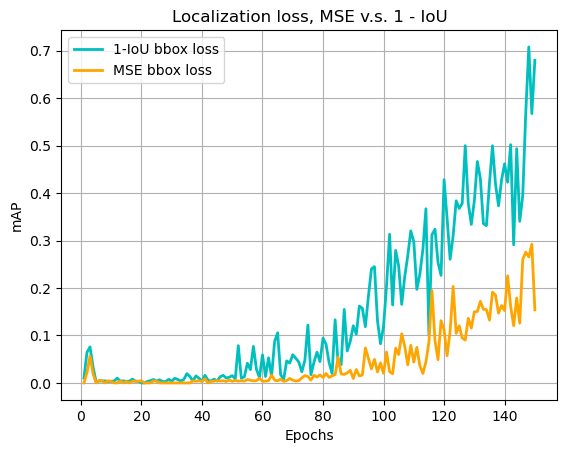
Figure 2: mAP on training set during 150 epochs. Blue curve uses 1 – IoU localization loss. Orange curve uses MSE loss on x, y, w, and h terms.
Because the loss terms in these 2 formulations are not directly comparable, it is more meaningful to compare the mAP scores. It seems that the MSE-loss version takes a longer time for the model to start converging, and the final result at the end of 150 epochs is also not as high as the 1 – IoU formulation.
It may be a bit puzzling to see this result. After all, if you manage to train the x/y locations as well as the width/height sizes to match, it automatically satisfies a minimum on 1 – IoU.
My interpretation on this: firstly, IoU is directly used in the final mAP metric, so we are directly teaching the network the exam questions.
Additionally, I guess by computing the 1 – IoU term as the loss function, we are linking the network with a “physical model” (although this simple IoU computation can barely be regarded as a “physical model”).
With MSE loss, we are forcing a direct match between the model outputs and target values. The MSE loss is the simplest form of direct match measurement, with perhaps the L1 loss as the only close match. With both L1 and L2 losses, we are asking the model: OK, whatever you do, get these number pairs as close as you can. We give no information whatsoever on how we would like the model to achieve such a goal. It is left for the model to figure out a way.
Maybe, by using this simple IoU formulation, we are laying out a more specific way for the model to follow along, and this specific way also happens to be the same way we gauge the model performance.
That is perhaps why achieving the x, y, w, h matches necessarily ensures a minimization on 1 – IoU, but actually achieving this is not as easy as directly targeting a maximization on IoU itself.
Calling IoU computation a “physical model” may not be quite appropriate, but you got the idea. I am aware that some people couple a neural network with a legit physical model, e.g. a numeric fluid simulator. On the other hand, people often complain that neural networks work as “black boxes”. Maybe it is partly because we are being too vague. Although complicated tasks like common CV problems almost entirely rule out rule-based solutions, maybe we can still be a bit more specific, at some places, at least?
4.2. 1 v.s. IoU objectness target
Objectness target values are controlled by setting the obj_loss argument to
'1 or 'iou'.
Results are given below.
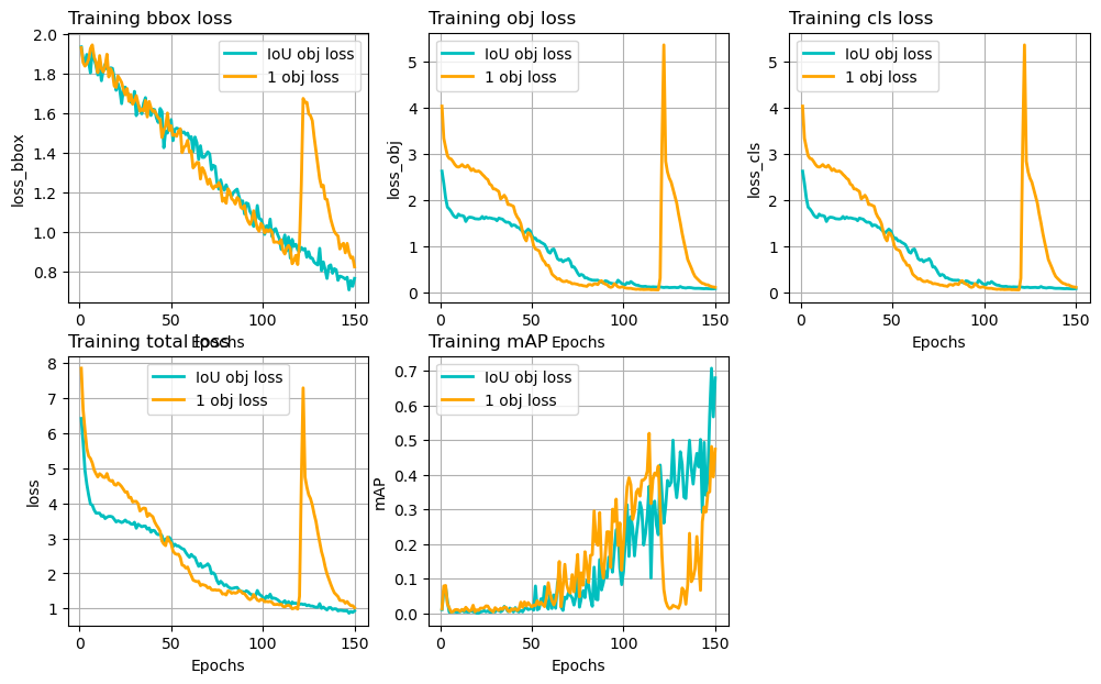
Figure 3: Different loss terms and mAP on training set during 150 epochs. Blue curve uses IoU as objectness target values. Orange curve uses 1.
This time, the training losses are comparable, so they are shown in addition to mAP.
The '1' objectness version has a faster convergence period during
about 50 – 100 epochs, compared with the 'iou' version. However, it
drops abruptly during epoch 120 – 130. This happened almost every time
I repeated the experiment. Although the mAP score recovers
quickly after epoch 130, it can’t reach as high as the 'iou'
version before the training terminates. I’m not sure what’s causing
this sudden degradation, but it does seem that this formulation is not quite
stable.
4.3. compute_loss() v.s. compute_loss2()
compute_loss() selects the “responsible” anchor
boxes by comparing ground truth labels with anchor box priors.
It is possible for more than 1 anchors in
different scales to be associated with a same label.
compute_loss2() compute the IoUs scores between labels and all 9
anchor boxes, and select the anchor with the highest IoU. It
is ensured that only 1 anchor box is associated with any label.
For both, I used IoU as localization loss and objectness targets.
Results are given below.
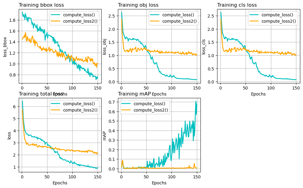
Figure 4: Different loss terms and mAP on training set during 150 epochs. Blue curve uses the compute_loss() function. Orange curve uses compute_loss2(). All other settings are the same.
For some reason, the compute_loss2() version stops improving after
about 20 epochs, and the mAP level stays close to 0 til the end of the
training. I am not sure what’s the problem, it could be my
coding mistakes. If you spot any please let me know.
5. Summary
This post develops the training code for YOLOv3. The loss function of YOLOv3 consists of 3 parts:
loss_box: errors from the bounding box predictions.loss_obj: errors from the objectness confidence score predictions.loss_cls: errors from the classification predictions.
The loss_obj term applies to all of the 10647 predictions per image in a
standard YOLOv3 model. This is far too big a number than the number of
objects in any training image. Therefore, it is important to counter
this positive-negative label imbalance.
The loss_box and loss_cls terms only apply to locations where
there is actually a ground truth label to predict. Finding these locations can be
a bit tricky, we eventually worked out 6 coordinates to achieve this:
\[(s, n, b, a, i, j)\]
where:
- \(s\): scale index, 0, 1, or 2.
- \(n\): label index, 0 to \(N-1\), \(N\) is the number of labels in the batch.
- \(b\): batch index, 0 to \(B-1\). \(B\) is the number of images in the batch.
- \(a\): anchor box index, 0, 1, or 2.
- \(i, j\): feature map cell location indices. Range depends on \(s\).
Having got these coordinates, we experimented computing the localization loss using:
- MSE losses on x, y, w and h terms of the bounding boxes, or
- 1 – IoU, where IoU is between predicted bounding boxes and ground truth labels.
Preliminary results suggest that method-2 works notably better.
We also experimented computing the objectness loss using:
- constant value 1 as objectness target, or
- IoU scores as objectness target.
Preliminary results suggest that method-2 works notably better.
The loss_cls loss is computed using Binary-Cross-Entropy losses.
We developed a train.py script that loads a small subset of the
COCO 2014 detection dataset, and trained a YOLOv3 model from
scratch, for 150 epochs. The best result (on training set itself) is
about mAP@0.5 = 0.7, and the model doesn’t appear to saturate at the
end of training.
This is just a toy example, but it shows that the training code works as expected, and you can use it to train on other datasets.
This concludes the Create YOLOv3 using PyTorch from scratch series. I learned a lot during the process. Reading something and thinking that you understand the subject can be the most misleading thing. Writing it out and making it work is a good test to verify one’s understanding. I might create more series on some other models in the future. Hope you have enjoyed this one.
Created: 2022-06-22 Wed 22:44


