Table of Contents
1. Overview
This would be the start of a mini-series, which talks about the inner workings of the YOLO Version 3 model, and how to construct one from scratch, using the PyTorch framework.
1.1. What is YOLO
For those not quite familiar with what the YOLO model is, YOLO (You Only Look Once) is a family of object detection neural network models that gains its reputation by fast inference time and a simple, end-to-end design. When it first came out in 2015, it was capable of performing real-time (> 30 fps) inference, while its major competitors (e.g. R-CNN, SSD) were still struggling at a level of a few fps. There are many follow-up improvements of the original YOLO model, including YOLOv2 and YOLOv3, both from its original creator Joseph Redmon. This series will be focusing on the YOLOv3 version.
But, in order to get to v3, we will be covering some necessary points in earlier versions. On the other hand, some aspects of the model have been changed during the v1 – v3 evolution, while others remained the same. I think I’ll mention some of the these points at relevant locations, and add some of my own interpretations, or interpretations from other people, to help make the point clearer. Or, if I’m unsure, I will also put down my questions, and if you could offer any help please leave a comment at the end.
1.2. Useful resources
Here are the original papers of the 3 versions of YOLO:
- YOLOv1 paper: You Only Look Once: Unified, Real-Time Object Detection.
- YOLOv2 paper: YOLO9000: Better, Faster, Stronger.
- YOLOv3 paper: YOLOv3: An Incremental Improvement.
Here are some helpful resources that I used as learning materials and references:
- C4W3LO9 YOLO Algorithm Youtube video, by Andrew NG
- How to implement a YOLO (v3) object detector from scratch in PyTorch: Part 1
- YOLOV3 Pytorch implementation by eriklindernoren
I won’t expect to outperform these authors, but only to offer yet another understanding and interpretation of the this wonderful model. Hopefully some of my own understandings about the model could turn out to be helpful to your learning process. And, writing it down in a relatively formal format also helps me gaining a deeper understanding of the subject. If you spot any mistakes in my posts please leave a comment at the end of the page.
1.3. Structure of the series
I’m planing to break down the entire series into a few parts:
- Understand the YOLO model: later part of this post. This will cover the building blocks inside the model, what are the model inputs and outputs, and the overall training and inference workflows.
- Build the model backbone. The backbone of YOLOv3 is a fully convolutional network called Darknet-53, which, as its name implies, has a total of 53 convolution layers. We will load the config file of the original YOLOv3 and implement it using PyTorch.
- Load pre-trained weights. To verify the Darknet-53 model we built works as intended, we could load the pre-trained YOLOv3 weights and perform some inferences on some images.
- Get the tools ready. Before getting into the training part, it might be helpful to first get some utilities ready, including the codes to compute IOU (Intersection-Over-Union), NMS (Non-Maximum suppression) and mAP (mean Average Precision).
- Training data preparation. This part will write some pre-processing codes to load the COCO detection dataset, including the images and annotation labels.
- Train the model. Whether to perform fine-tuning, or train a new model on a different type of data from scratch, we need to have properly working training codes. This is, in my opinion, a lot harder than all the previous parts, so I left it at the very end.
I plan to write up and publish the posts one-by-one. So please stay tuned if you find these helpful or interesting. (I don’t know how to set up notifications or subscription system. Apologies.)
2. Understand the YOLO model
2.1. What does YOLO do
In a nutshell, the YOLO model takes an image, or multiple images, and detects objects in the images. The output of the model consists of:
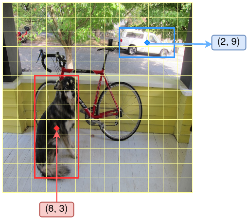
Figure 1: Demontration of the YOLOv3 detection result. The thin yellow grid lines divide the entire image into 13 * 13 cells. Each cell makes its own predictions. 2 detected objects, the dog and the truck, are shown by their bounding boxes. The center of the dog box is located in the cell (8, 3), and the center of the truck box is located in cell (2, 9). Note that I made up these boxes and locations for illustration purposes, the truth values of this sample may be somewhat different. But the principle is the same.
- A number of objects it recognizes, it could be 1, or many, or none.
- For each recognized object, it outputs:
- Its x- and y- coordinates and the width and height of the bounding box enclosing the object. Using these coordinate and size information, one could locate the detected object in the image, and visualize the detection by drawing out the bounding box on top of the image, as in the example in Figure 1.
- A confidence score measuring how confidence the model is about the existence of this detected object. This is a score in the range of 0 – 1, and could be used to filter out those less certain predictions.
If the model is trained on data containing multiple types of objects, or, using a more formal phrase, multiple classes of objects, it also outputs a confidence score for the detected objecting belonging to each class. Typically these classes are mutually exclusive, i.e. an object belongs to only 1 class (a multi-class problem). But a variant of the YOLOv2 – YOLO9000 – was designed to be able to detect objects belongs to more than 1 classes (a multi-label problem). E.g. a Norfolk terrier is labeled both as a “terrier” and as a “dog”.
In our subsequent discussion and implementation, we will be restricted to the multi-class model: the classes are mutually exclusive.
So, the model performs multiple tasks, localization and classification, in a single pass through the network, thus its name You Only Look Once. This also makes YOLO a multi-task model.
2.2. Input and output data
Given the above, the input data to the YOLO model are the images. When represented in numerical format, these are N-dimensional arrays/tensors of the shape:
[Bt, C, H, W]
where,
Bt: batch-size.C: size of the channel or feature dimension. For images in RGB format,C = 3. The ordering of the 3 color channels doesn’t really matter, as long as you stick to the same ordering during training and inference time.HandWare the height and width of the image, in number of pixels. These need to be standardized to a fixed size, e.g.416 x 416, or take some random perturbations as a method of data augmentation method during the training state, e.g. randomly sampled within a range. But typically one has to set a reasonable upper bound during training time, to save computations.
Also note that this [Bt, C, H, W] ordering is following the PyTorch
convention. In Tensorflow it is ordered as [Bt, H, W, C].
When making inferences/predictions, the model outputs a number of detection proposals, because there could be multiple objects in a single image. How these proposals are arranged will be covered in just a minute. But we could already make an educated guess about what each proposal would contain. Based on the previous section, it should provide an array like this:
[x, y, w, h, obj, c1, c2, ..., ck]
where,
x,y: give information about the x- and y- coordinates of the detection.w,h: are the width and height information.obj: is the object confidence score.c1tock: the confidence score for each class.
Therefore, each proposed object detection is an array/tensor of length 5 + Nc, where Nc is the number of classes to classify the detected object.
For instance, the COCO detection dataset has 80
different classes, then Nc = 80, and each detection is represented
by a tensor of size 5 + 80 = 85.
For the Pascal VOC dataset, Nc = 20, and each detection is a
tensor of size 5 + 20 = 25.
The ordering of the x, y etc. elements are not crucial as long as
it is kept consistent. But I also don’t see any good reason to break
this convention, so I will use this same ordering as the original YOLO model.
2.3. Arrange the detections, horizontally
The reasoning is fairly intuitive.
There are typically multiple objects in a single image, so we need to make multiple predictions.
Different objects are located at different places in the image, so we place different detections at different locations.
In the realm of numerically represented images, it is most natural to encode locations as elements in a matrix/array.
That’s how YOLO deals with this: it divides a “prediction matrix/array”
into Cy number of rows and Cx number of columns, so a total of
Cy * Cx cells, and each cell makes its own predictions,
corresponding to different places in the image.
In the example shown in Figure 1, the thin grid lines denote such
cells, and the dog target object is bounded by a bounding box, whose
center point is located in cell (8,3). Another object, the truck,
is located at a different cell (2,9).
2.4. Multiple detections in the same cell
A natural question to ask is: what if two objects overlap with each other and are located into the same cell?
One way to solve this problem is to make the cell size smaller, to reduce the chance that multiple objects would land in the same cell. This is particularly effective for large-sized objects.
Additionally, YOLO also allows each cell to predict multiple objects. And this is done slightly differently in YOLOv1 and later versions (up to v3 at least, I haven’t read about v4 or later).
In YOLOv1, each cell makes B number of predictions, corresponding to
B number of bounding boxes. For instance, for evaluation on the Pascal VOC
data, the author set B = 2. So the total number of predictions is
Cy * Cx * B. But, the B number of predictions in each cell have to be of the same class, so the output tensor size is [Cy, Cx, B * 5 + Nc].
Since YOLOv2, the concept of anchor boxes was introduced. These
could be understood as prescribed bounding box templates. They come
as different sizes and aspect ratios. For instance, one of them used
in YOLOv3 has a dimension of 116 * 90, measured in number of pixels. We will
go deeper into the size computation shenanigans later, but for now, it
is suffice to know that each cell can produce more than 1 objects. In
YOLOv1, each prediction is associated with a bounding box. In later
versions, each prediction is associated with an anchor box.
The number of anchor boxes B in each cell can be changed. In YOLOv2 they
used 5, and in YOLOv3 3. Different from v1, the B number of
predictions in each cell can be of different classes in v2 and later
versions. So, the output tensor size is now [Cy, Cx, B, 5 + Nc].
2.5. Multi-scale detections
The author of YOLO admitted that the v1 version struggled at detection small objects, particularly those come in groups:
Our model struggles with small objects that appear in groups, such as flocks of birds.
(From the YOLOv1 paper.)
Why is it the case?
The limited number of bounding boxes in each cell, and the relatively small number of predicting cells mentioned previously are part of the reason.
It is also because the network of YOLOv1 makes predictions using the outputs only from the last model layer.
Because the information from input images have gone through multiple convolution layers and pooling layers, the feature map sizes are becoming smaller and smaller in the width and height dimensions. What are left at the end of the convolution layers are highly distilled representations of the image, with fine-grain details largely lost during the process. And small-sized objects are particularly susceptible to such a loss.
So, to counter this, YOLOv2 included a passthrough layer that
connects feature maps with a 26 * 26 resolution with those with
13 * 13 resolution, thus providing some fine-grained features to the
detection-making layers. The connection is done in a pixel-shuffle
manner. We will not expand on this because YOLOv3 does this
differently.
YOLOv3 achieves multi-scale detections, by producing predictions at 3 different scale levels:
- Large scale: for the detection of large-sized objects. These outputs
are taken at the end of the convolution network (see Figure 2 for
a schematic), with a stride of
32. I.e. if the input image is
416 * 416pixels, feature maps at stride-32 have a size of416 / 32 = 13. - Mid scale: for detecting mid-size objects. These are taken from
the middle of the network, with a stride of 16. I.e. feature maps
are
26 * 26. - Small scale: for detecting small-sized objects. These are taken
from an even earlier layer in the network, with a stride of
8. I.e. feature maps are
52 * 52.
Again, to complement the mid scale and small scale detections with fine-grained features, passthrough connections are made:
- For mid scale detections, feature map from a layer towards the end of the network is taken. These feature maps are at stride-32 (13 * 13 in size). Up-sample them (by interpolation) by a factor of 2, to a stride-16 (26 * 26 in size). Then concatenate them with feature map from the last layer with stride=16 (layer number 61) along the channel dimension. This concatenated feature map is passed through a few layers of convolutions before outputting a prediction.
- For small scale detections, feature map from the above created side-branch at stride-16 is taken, up-sampled to stride=8, and concatenated with the output from layer 36 at a stride of 8. This concatenated feature map is passed through a few more conv layers before outputting the prediction for small objects.
Figure 2 below gives an illustration of this process. Note that when making the small scale predictions, it is incorporating information at 3 scales: stride 8, 16 and 32.
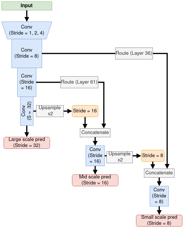
Figure 2: Structure of the YOLOv3 model. Blue boxes represent convolution layers, with their stride level labeled out. Prediction outputs are shown as red boxes, and there are 3 of them, with different stride levels. Pass-through connections are labeled as “Route”, and the layer from which these are taking out are put in parenthese (e.g. Layer 61. Indexing starts from 0).
This method allows us to get more meaningful semantic information from the upsampled features and finer-grained information from the earlier feature map.
(From the YOLOv3 paper.)
So, with 3 scales, the output tensor size is now [Cy1, Cx1, B, 5 +
Nc] + [Cy2, Cx2, B, 5 + Nc] + [Cy3, Cx3, B, 5 + Nc].
Where Cy1 = Cx1 = 13, Cy2 = Cx2 = 26 and Cy3 = Cx3 = 52.
Recall that in YOLOv3, B=3 number of prescribed anchor boxes are associated with
each scale level, these are:
(116, 90), (156, 198), (373, 326)for large objects,(30, 61), (62, 45), (59, 119)for mid objects,(10, 13), (16, 30), (33, 23)for small objects.
These are taken from a K-Means clustering of the bounding boxes from training data. And the numbers are using the unit of pixels. This leads to size and location computations, detailed in the following sub-section.
2.6. The localization task
Let’s dive deeper into how YOLO predicts the location of an object.
Firstly, the location of an object is represented by the location of its bounding box, so we need only 4 numbers, in either of these 2 ways:
- (x, y) coordinate of a corner point and (x, y) coordinate of the
diagonal point:
[x1, y1, x2, y2]. Or - (x, y) coordinate of the center point and (width, height) size:
[x, y, w,
   h]
.
YOLOv3 takes the 2nd [x, y, w, h] representation for bounding
box predictions.
But both formats will be used at different places, so we need some housekeeping codes
to do the transitions. It should be trivial to implement though.
Now about the sizes. I found it beneficial to first get the coordinate systems straight. Because YOLO implicitly uses 3 different coordinate systems, it is easy to get confused about which one is used at different places, particularly during the training stage.
- The original, image coordinate: measured in pixels. This is the coordinate system we use to locate a pixel in an image, x- for counting the columns, and y- for rows.
- The feature map coordinate: again, x- for counting columns and y-
for rows, but here we are counting the feature map cells.
Recall that we used the term cells previously, it may
be beneficial to stick to this cells term to distinguish from the
pixels unit used in the image coordinate. This distinction is
easily observed in Figure 1, where the image is divided
into
13 * 13cells, but one such cell obviously contains more than 1 pixels. At stride=32, the feature map has a size13 * 13. So the feature map coordinate at this particular stride level measures offsets within a13 * 13matrix. Similarly, at stride=16, the feature map measures offsets within a26 * 26matrix, and 1 unit of offset here is twice as large as 1 unit of offset at the stride=32 level, in the image coordinate distance sense. Also note that offsets in feature map coordinate can have decimal places. E.g.1.5means 1 and a half units of offset, with respect to the corner point of the feature map at a certain stride level. - The fractional coordinate: for both x- and y- dimensions,
this is a positive float. It could be measuring
offsets, like the x- and y- locations, or width/height
sizes. For instance, the bounding box labels in training data are
often encoded in fractional coordinates. E.g. in the COCO
detection data, a label
is in
[x_center, y_center, width, height, class]format, and has values of[0.5, 0.51, 0.1, 0.12, 10], then the first 4 floats tell the bounding box location/size measured in fractions of that image.
Now let’s look at how YOLOv3 locates a bounding box.
First, this is the equation given in the YOLOv2 paper (same holds for YOLOv3):
\begin{equation} \begin{aligned} b_x = & \sigma(t_x) + c_x \\ b_y = & \sigma(t_y) + c_y \\ b_w = & p_w e^{t_w} \\ b_h = & p_h e^{t_h} \\ \end{aligned} \end{equation}where:
\(t_y\), \(t_x\) are the raw model outputs about the y- and x- locations of the bounding box, produced by a cell at location \((c_y, c_x)\) in the feature map.
\(\sigma()\) is the sigmoid function. So \(\sigma(t_y)\) and
\(\sigma(t_x)\) are floats in the [0,1] range, and are fractional
offsets with respect to the corner of the cell at \((c_y, c_x)\).
When added onto the integer cell counts of \(c_y\) and \(c_x\), the resultant bounding box center location \((b_y, b_x)\) is using the feature map coordinate system.
\(t_w\) and \(t_h\) are the raw model outputs about the width and height sizes of the bounding box, again produced by the same cell at \((c_y, c_x)\) in the feature map.
\(p_w\) and \(p_h\) are the width and height of an anchor box, so \(e^{t_w}\) and \(e^{t_h}\) are in the factional coordinate, and act as non-negative scaling factors to resize this associated anchor box to match the object being detected. Because \(b_x\) and \(b_y\) are in feature map coordinates, so should \(b_w\) and \(b_h\).
But, the prescribed anchor boxes, e.g. the one with a size of (116,
90), are measured in image coordinates using units of pixels.
Therefore, we need to convert 116 to a width measure in the feature
map coordinate, and similarly for the height of 90. To do so, we
need to divide them by the stride of the feature map in
question. For instance, for large scale detections, \(p_w\) may be \(116
/ 32 = 3.625\) and \(p_h\) may be \(90 / 32= 2.8125\).
But why “may be”? Recall that a single cell has 3 anchor boxes in YOLOv3,
so it could have been the anchor box of (156, 198), or the (373,
326) one, in the case of large scale detections. During inference
time, all 3 anchor boxes are used. During training time, only those
with the closet match with the ground truth label will be picked. If
the ground truth label object is not a “large” object in the first
place, maybe none of the 3 are picked. We will come back to the
training process in a later post.
Hopefully I’m not over-complicating things, but I found it helpful to map out these different coordinate systems to better understand YOLO’s localization mechanisms.
*Figure 3 below gives an illustration of the relationships between the 3 coordinate systems, and the conversions of some variables in between them.
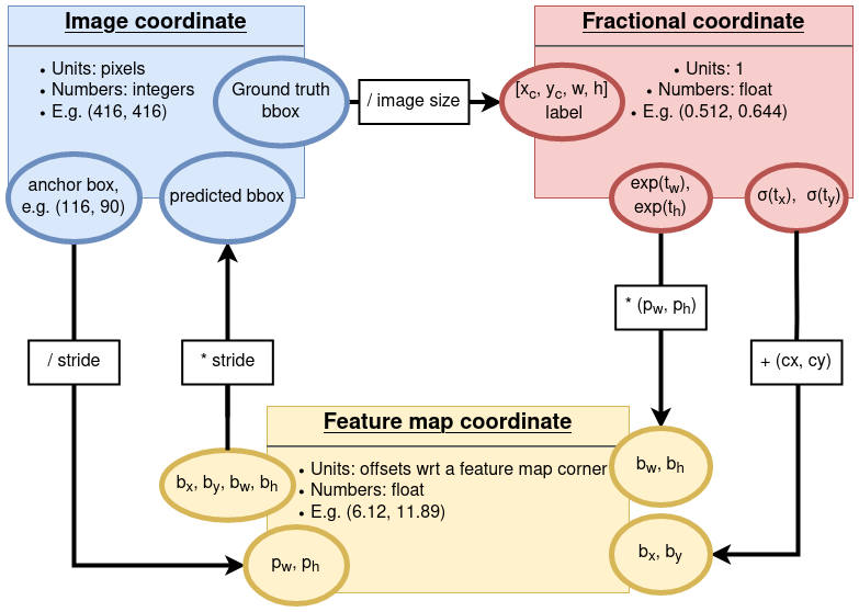
Figure 3: Relationships between the 3 coordinate systems used in YOLOv3. Ellipses show some variables in the coordinate system as the corresponding color, and arrows denote operations applied to convert from 1 coordinate to another.
Having got the predictions in [bx, by, bw, bh] format, we only need
to multiply with the current stride level to get back to the image
coordinate, measured in pixels, and the results could be plotted out.
(NOTE that if you have re-sized the image, for instance, to the
standard 416 * 416 size, there is an extra step of re-scaling needed.)
So that is, very superficially, how YOLOv3 predicts object locations. Exactly
how it produces the correct numbers of [tx, ty, tw, th] such that
simple coordinate transformations could lead to a correct bounding box
is beyond me. And frankly, I don’t think we understand neural networks
well enough to clearly decipher this black-box. All we can say is that
when we feed the model with enough number of correctly formulated training data, it
somehow learns to build the correct associations, with certain degrees
of generalizability beyond the data it has seen.
2.7. Confidence and classification scores
In addition to localization, YOLO also predicts a confidence score of
the existence of an object, and a probability for the objecting
belonging to each of the Nc possible classes, should there being an
object in the first place.
Formally, the equation for confidence score prediction is:
\[ P_o = \sigma(t_o) \]
where \(t_o\) is the raw model output. Using the
[x, y, w, h, obj, c1, c2, ..., ck]
arrangement, it is the obj term.
Again, \(\sigma()\) is the sigmoid function, and its output can be interpreted as a probability prediction.
The probability prediction for classes is a conditioned on the objectness score:
Pr(Class_i | Object) * Pr(Object)
Note that this is the equation (1) in the YOLOv1 paper, and it is stated that:
At test time we multiply the conditional class probabilities and the individual box confidence predictions,
Pr(Classi |Object) ∗ Pr(Object) ∗ IOU(truth, pred) = Pr(Classi) ∗ IOU(truth, pred)
I’m wondering if there is some error in this statement: we don’t
really have the truth term to compare against at test time. Based
on the implementation of YOLOV3 Pytorch implementation by
eriklindernoren, I assume that there shouldn’t be an IOU term at
test/inference time.
Again, under the exclusive classes assumption, class prediction is just a multi-class classification task, and the only difference is the conditional probability of objectness prediction that is multiplied by.
I think I’ll talk more about objectness and class predictions in the Training the model post later.
3. Summary
The above talked about in the expected configurations, how a well- trained YOLOv3 model makes detections. Let’s summarize the main points.
- YOLOv3 makes predictions at 3 scale levels: for large objects, mid objects, and small objects.
- The 3-scale predictions come from feature maps at 3 stride levels: stride-32 for large objects, stride-16 for mid objects, and stride=8 for small objects.
At each scale level, there are 3 prescribed anchor boxes:
(116,
90)
, (156, 198), (373, 326)for large objects,(30, 61), (62, 45), (59, 119)for mid objects,(10, 13), (16, 30), (33, 23)for small objects.
These are taken from a K-Means clustering on the bounding boxes from training data, and all sizes are measured in the image coordinate, in pixels.
- At each scale level, the model predicts x- and y- location
(bx, by)of a bounding box as offsets wrt the corner of the feature map. And width and height of the bounding box,(bw, bh), again wrt to the size of the corresponding feature map. - To get back to the image coordinate measured in pixels, we
multiple the
[bx, by, bw, bh]values by the stride level of the feature map: 32 for large scale objects, 16 for mid, and 8 for small objects. - In addition to locations, the model also predicts a confidence score about the existence of an object inside that bounding box we
just formulated. And, for each of the prescribed
Ncnumber of classes, a conditioned probability of the object belonging to that class.
That’s the part of the work involving the YOLO model itself. There are some extra housekeeping steps afterwards:
- Thresholding the confidence scores: the model may produce a large number of low confidence predictions, which could be filtered out using a threshold on the confidence scores.
- Removing duplicates by Non-maximum suppression: the model may produce multiple similar predictions around the true location of an object, with slightly different confidence levels. Without further information, it is reasonable to assume that the one with highest confidence score is the “correct” prediction, while other highly overlapping bounding boxes are “duplicated predictions”. Such duplicates are typically removed using a Non-maximum suppression method. We will implement this in a later post.
Figure 4 shows a schematic layout of the YOLOv3 model, summarizing much of the key points in this post.
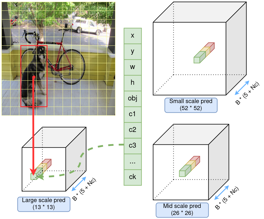
Figure 4: Schematic layout of a YOLOv3 model predictions. Predictions at 3 scales are represented by 3 cubes, with different row/column numbers, but the same size in the channel dimension. In each scale, a cell in the feature map is highlighted. Each cell consists of predictions from 3 anchor boxes, represented by 3 different colors. The identified object, the dog, is hyperthetically predicted by the green anchor box, at a certain cell, in the large scale prediction cube.
That’s pretty much it for the 1st part of the series. Hopefully this makes things a bit clearer if you are interested in the YOLO model. We’ll revisit some of these points in later posts, with code implementations. The next part will be building the Darknet-53 network. So please stay tuned.
Created: 2022-06-22 Wed 22:36


