Table of Contents
1. What’s this about
This post is modified from one of my reading notes and coding practices.
The original paper is: Ladd, Daniel W., 1975: An Algorithm for the Binomial Distribution with Dependent Trials.
If the outcomes of a sequence of trials can be assumed to be independent of each other, then the number of successes \(j\) in a total of \(K\) trials, each with a probability of success \(P\) is modeled as a binomial distribution:
\[ Pr(j, K; P) = \left(\begin{array}{c}K\\ j\end{array}\right) P^j (1-P)^{K-j} \]
This article is concerned with the distribution when the independent constraint is relaxed, and the trials are assumed to be dependent of each other, by a “one-stage dependence”, i.e. the outcome of one trials affects the outcome of the next, and no others.
In this post I will cover:
- the formulation of the problem,
- the formulae for the probability mass function and cumulative distribution function,
- a Python implementation, with Cython acceleration for one of the functions,
- some preliminary distribution comparisons between the dependent and independent assumptions.
2. Formulation of the problem
Let \(X_i\) be a sequence of random variables, each \(X_i\) takes the value \(0\) or \(1\):
\[ P = Pr(X_i=1) \; for \; any \; i. \]
The sequence of \(X_i\) forms a Markov chain, with the following conditional probabilities:
\[ \left\{\begin{matrix} & P_{hh} =& Pr(X_i=1 | X_{i-1} =1), \\ 1-P_{hh} =& P_{mh} =& Pr(X_i=0 | X_{i-1}=1), \\ & P_{hm} =& Pr(X_i=1 | X_{i-1}=0), \\ 1-P_{hm} =& P_{mm} =& Pr(X_i=0 | X_{i-1}=0) \\ \end{matrix}\right. \]
For a particular \(i=n\), let \(P_n = Pr(X_n=1)\), and \(P_{n-1} = P = P_n\).
For the Markov model, one has \(P_n = P_{n-1} P_{hh} + (1 – P_{n-1})P_{hm}\).
This leads to \(P = P P_{hh} + (1-P) P_{hm}\), and:
\begin{equation} \label{org73c46b2} P_{hh} = 1 – \frac{1-P}{P} P_{hm} \end{equation}Thus, the 4 conditional probabilities:
- \(P_{hh}\)
- \(P_{mm}\)
- \(P_{hm}\)
- \(P_{mh}\)
are determined from a specified value of \(P\), and either \(P_{hm}\) or \(P_{hm}\).
Denote the probability of having \(j\) hits in \(K\) trials as:
\[ \Phi_{j,K} (P, P_{hh}) \]
or
\[ \Phi_{j,K} (P, P_{hm}) \]
For either case, use \(\Phi_{j,K}\) as a shorthand.
Denote the probability of having \(j\) or fewer successes:
\begin{equation} \label{org4933a54} S(K, j; P) = \sum_{i=0}^{j} \Phi_{i,K} \end{equation}3. The solution schematic
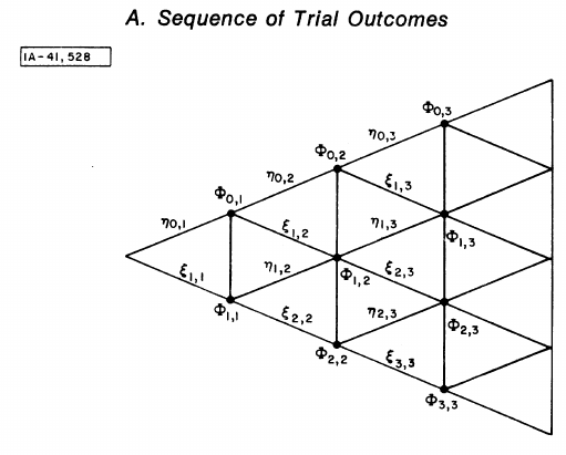
Figure 1: Figure A from Ladd 1975. The schematic representation of the various outcomes of a series of trials.
To read the schematic:
- Each vertical line represents one trial.
- Nodes on the lines are the possible numbers of successes, from \(0\) on the top to \(K\) on the bottom.
- To each any point, e.g. \(\Phi_{2,3}\) on the graph, one goes from the left to the right.
Using the Markov chain assumption, the probability of \(\Phi_{j,K}\) depends on the probabilities of the immediate previous trial. Formally, this is:
\begin{equation} \label{orgf56ec61} \Phi_{j,K} = \eta_{j,K} + \xi_{j,K} \end{equation}where:
- \(\eta_{j,K} \equiv Pr(\text{j successes in K trials, the Kth one fails})\). This is graphically represented as an upward edge pointing from the left towards the point \(\Phi_{j,K}\).
- \(\xi_{j,K} \equiv Pr(\text{j successes in K trials, the Kth one succeeds})\). This is graphically represented as a downward edge pointing from the left towards the point \(\Phi_{j,K}\).
Equation \eqref{orgf56ec61} defines the transitional relationships. Here are the starting values:
\begin{equation} \left\{\begin{matrix} \eta_{0,1} =& 1-P \\ \eta_{1,1} =& 0 \\ \Phi_{0,1} =& 1-P \\ \xi_{0,1} =& 0 \\ \xi_{1,1} =& P \\ \Phi_{1,1} =& P \\ \end{matrix}\right. \end{equation}Then, the general solution is:
\begin{equation} \label{org51d9b00} \left\{\begin{matrix} \eta_{0,K} =& \eta_{0,K-1}P_{mm} = (1-P) P_{mm}^{K-1} \\ \xi_{0,K} =& 0 \\ \eta_{j,K} =& \xi_{j,K}P_{mh} + \eta_{j,K-1}P_{mm} \\ \xi_{j,K} =& \eta_{j-1,K-1}P_{hm} + \xi_{j-1,K-1}P_{hh},\; (j=1,2,\cdots,K-1) \\ \eta_{K,K} =& 0 \\ \xi_{K,K} =& \xi_{K-1,K-1}P_{hh} = P P_{hh}^{K-1} \\ \end{matrix}\right. \end{equation}
4. Python implementation
4.1. Recursive version
It is noticed that \eqref{org51d9b00} is written in a recursive manner, therefore it is most natural to code it using also recursive functions. Below is the Python implementation.
Firstly, the pmf() function that computes the probability mass function:
import numpy as np

def pmf(j, k, p, phh=None, phm=None):
    '''Compute the probability mass function binomial distr with dependent
    trials, recursive version

    Args:
        j (int): number of successes.
        k (int): number of trials.
        p (float): probability of any trial being success.
    Keyword Args:
        phh (float): probability of success given its previous trial is success.
        phm (float): probability of success given its previous trial is fail.
            <phh> and <phm> must be provided at least one. If both are given, <phm>
            is computed from <phh>.
    Returns:
        res (float): probability of j successes in k trials.
    '''
    assert j >= 0, "<j> must >= 0."
    assert k >= 0, "<k> must >= 0."
    assert p >= 0, "<p> must >= 0."

    if j == 0 and k == 1:
        return 1 - p
    if j == 1 and k == 1:
        return p

    if phh is None and phm is None:
        raise Exception("Either <phh> or <phm> must be provided.")

    if phh is None:
        phh = 1 - (1-p) / p * phm
    else:
        phm = (p - p*phh) / (1 - p)

    pmh = 1 - phh
    pmm = 1 - phm
    f_jk = compute_jkf(j, k, p, pmm, pmh)
    s_jk = compute_jks(j, k, p, phh, phm)
    res = f_jk + s_jk

    return res
The pmf() function calls 2 additional functions:
compute_jkf(): computes the \(\eta_{j,K}\) term.compute_jks(): computes the \(\xi_{j,K}\) term.
These 2 are the recursive functions:
from functools import lru_cache

@lru_cache(maxsize=1024)
def compute_jkf(j, k, p, pmm, pmh):
    '''Compute the probablity of j successes in k trials, with the kth one fails

    Args:
        j (int): number of successes.
        k (int): number of trials.
        p (float): probability of any trial being success.
        pmm (float): probability of fail given its previous trial is fail.
        pmh (float): probability of fail given its previous trial is success.
    Returns:
        res (float): probability of j successes in k trials, with the kth one fails.
    '''

    if j == 0 and k == 1:
        return 1 - p
    if j == 1 and k == 1:
        return 0
    if j == 0:
        return (1 - p) * pmm**(k-1)
    if j == k:
        return 0

    phh = 1 - pmh
    phm = (p - p*phh) / (1 - p)
    return compute_jks(j, k-1, p, phh, phm) * pmh + compute_jkf(j, k-1, p, pmm, pmh) * pmm

@lru_cache(maxsize=1024)
def compute_jks(j, k, p, phh, phm):
    '''Compute the probablity of j successes in k trials, with the kth one succeeds

    Args:
        j (int): number of successes.
        k (int): number of trials.
        p (float): probability of any trial being success.
        phh (float): probability of success given its previous trial is success.
        phm (float): probability of success given its previous trial is fail.
    Returns:
        res (float): probability of j successes in k trials, with the kth one succeeds.
    '''

    if j == 0 and k == 1:
        return 0
    if j == 1 and k == 1:
        return p
    if j == 0:
        return 0
    if j == k:
        return p * phh**(k-1)

    pmh = 1 - phh
    pmm = 1 - phm

    return compute_jkf(j-1, k-1, p, pmm, pmh) * phm + compute_jks(j-1, k-1, p, phh, phm) * phh
Note that we are using the lru_cache decorators to cache
intermediate results. I have another post that talks a bit more on
caching and lazy evaluation.
Now a simple test run: when \(P_{hh} = 0.5\), i.e. one successful trial infers
no bias for the next one, it should fall back to a binomial
distribution. So we compare the result with that from scipy.stats.binom:
K = 100
j = 50
p = 0.5
phh = 0.5

prob1 = pmf(j, K, p, phh)
print(prob1)

from scipy.stats import binom
prob2 = binom.pmf(j, K, p)
print(prob2)
The output:
0.0795892373871788
0.07958923738717875
The above recursive implementation works all fine for relatively small-sized problems, but will fail once the \(K\) number goes large.
This is because Python’s recursion depth is quite limited, to about 1000. Recursive functions (including tail-recursions) will fail if the stack is full. See the below example call:
# large scale, recursive version
K = 1000
j = 5
p = 0.5
phh = 0.5

prob = pmf(j, K, p, phh)
print(prob)
Running the above snippet will trigger the following error:
Traceback (most recent call last):
  File "dependent_binomial.py", line 318, in <module>
    prob4 = pmf(j, K, p, phh)
  File "dependent_binomial.py", line 52, in pmf
    f_jk = compute_jkf(j, k, p, pmm, pmh)
  File "dependent_binomial.py", line 84, in compute_jkf
    return compute_jks(j, k-1, p, phh, phm) * pmh + compute_jkf(j, k-1, p, pmm, pmh) * pmm
  File "dependent_binomial.py", line 112, in compute_jks
    return compute_jkf(j-1, k-1, p, pmm, pmh) * phm + compute_jks(j-1, k-1, p, phh, phm) * phh
  File "dependent_binomial.py", line 84, in compute_jkf
    return compute_jks(j, k-1, p, phh, phm) * pmh + compute_jkf(j, k-1, p, pmm, pmh) * pmm
  File "dependent_binomial.py", line 112, in compute_jks
    return compute_jkf(j-1, k-1, p, pmm, pmh) * phm + compute_jks(j-1, k-1, p, phh, phm) * phh
  File "dependent_binomial.py", line 84, in compute_jkf
    return compute_jks(j, k-1, p, phh, phm) * pmh + compute_jkf(j, k-1, p, pmm, pmh) * pmm
  File "dependent_binomial.py", line 112, in compute_jks
    return compute_jkf(j-1, k-1, p, pmm, pmh) * phm + compute_jks(j-1, k-1, p, phh, phm) * phh
  File "dependent_binomial.py", line 84, in compute_jkf
    return compute_jks(j, k-1, p, phh, phm) * pmh + compute_jkf(j, k-1, p, pmm, pmh) * pmm
  File "dependent_binomial.py", line 112, in compute_jks
    return compute_jkf(j-1, k-1, p, pmm, pmh) * phm + compute_jks(j-1, k-1, p, phh, phm) * phh
  File "dependent_binomial.py", line 84, in compute_jkf
    return compute_jks(j, k-1, p, phh, phm) * pmh + compute_jkf(j, k-1, p, pmm, pmh) * pmm
  File "dependent_binomial.py", line 84, in compute_jkf
    return compute_jks(j, k-1, p, phh, phm) * pmh + compute_jkf(j, k-1, p, pmm, pmh) * pmm
  File "dependent_binomial.py", line 84, in compute_jkf
    return compute_jks(j, k-1, p, phh, phm) * pmh + compute_jkf(j, k-1, p, pmm, pmh) * pmm
  [Previous line repeated 486 more times]
  File "dependent_binomial.py", line 112, in compute_jks
    return compute_jkf(j-1, k-1, p, pmm, pmh) * phm + compute_jks(j-1, k-1, p, phh, phm) * phh
  File "dependent_binomial.py", line 72, in compute_jkf
    if j == 0 and k == 1:
RecursionError: maximum recursion depth exceeded in comparison
It is possible to enlarge this maximum recursion depth. But I will illustrate another way, which is to change the recursive calls into for loops.
4.2. Non-recursive version
Referring back to the schematic in Figure 1, it is noticed that to get to a certain point \(\Phi_{j,K}\) on the graph, it works from the left most end to the right.
We can re-draw the schematic graph in a slightly different way, as shown in Figure 2 below:
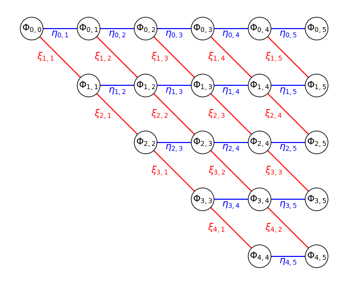
Figure 2: Similar solution schematic in Figure 1 drawn on a regular grid.
We put all the target nodes of \(\Phi_{j,K}\) on a regular grid, and draw the \(\eta_{j,K}\) transitions as blue, horizontal edges, and \(\xi_{j,K}\) transitions as red, diagonal edges.
From Equations \eqref{org51d9b00}, it is further noticed that we only take a top-down step in the computation of \(\xi_{j,K} = \eta_{j-1,K-1}P_{hm} + \xi_{j-1,K-1}P_{hh}\). The computation of \(\eta_{j,K} = \xi_{j,K}P_{mh} + \eta_{j,K-1}P_{mm}\) then only takes a left-right step from \(K-1\) to \(K\).
So, we will be building 2 2D arrays, one for \(\eta\) and one for \(\xi\) terms, both with only the upper triangle filled. \(j\) will be the row index, and \(K\) the column index.
Here is the non-recursive version:
def compute_jksf(j, k, p, pmm, pmh, phh, phm):
    '''Compute the transition probabilities leading to the prob of j successes in k trials

    Args:
        j (int): number of successes.
        k (int): number of trials.
        p (float): probability of any trial being success.
        pmm (float): probability of fail given its previous trial is fail.
        pmh (float): probability of fail given its previous trial is success.
        phh (float): probability of success given its previous trial is success.
        phm (float): probability of success given its previous trial is fail.
    Returns:
        farr (ndarray): 2d array with shape (k+1, k+1), the (j,k) element is the
            probability of j successes in k trials and the kth one is fail.
        sarr (ndarray): 2d array with shape (k+1, k+1), the (j,k) element is the
            probability of j successes in k trials and the kth one is success.
    '''

    farr = np.zeros([k+1, k+1])
    sarr = np.zeros([k+1, k+1])
    for kk in range(1, k+1):
        for jj in range(0, kk+1):
            if jj == 0:
                sjk = 0
                fjk = (1-p) * pmm**(kk-1)
            elif jj == kk:
                sjk = p * phh**(kk-1)
                fjk = 0
            else:
                sjk = farr[jj-1, kk-1] * phm + sarr[jj-1, kk-1]*phh
                fjk = sarr[jj, kk-1] * pmh + farr[jj, kk-1] * pmm
            farr[jj,kk] = fjk
            sarr[jj,kk] = sjk

    return farr, sarr
The \(\xi_{j,K}\) term is computed using:
sjk = farr[jj-1, kk-1] * phm + sarr[jj-1, kk-1]*phh
And the \(\eta_{j,K}\) term is computed using
fjk = sarr[jj, kk-1] * pmh + farr[jj, kk-1] * pmm
This compute_jksf() function will be called by a new pmf2()
function to compute the probability mass function:
def pmf2(j, k, p, phh=None, phm=None):
    '''Compute the probability mass function binomial distr with dependent
    trials, non-recursive version

    Args:
        j (int): number of successes.
        k (int): number of trials.
        p (float): probability of any trial being success.
    Keyword Args:
        phh (float): probability of success given its previous trial is success.
        phm (float): probability of success given its previous trial is fail.
            <phh> and <phm> must be provided at least one. If both are given, <phm>
            is computed from <phh>.
    Returns:
        res (float): probability of j successes in k trials.
    '''

    assert j >= 0, "<j> must >= 0."
    assert k >= 0, "<k> must >= 0."
    assert p >= 0, "<p> must >= 0."

    if j == 0 and k == 1:
        return 1 - p
    if j == 1 and k == 1:
        return p

    if phh is None and phm is None:
        raise Exception("Either <phh> or <phm> must be provided.")

    if phh is None:
        phh = 1 - (1-p) / p * phm
    else:
        phm = (p - p*phh) / (1 - p)

    pmh = 1 - phh
    pmm = 1 - phm
    f_jk, s_jk = compute_jksf(j, k, p, pmm, pmh, phh, phm)
    res = f_jk[j, k] + s_jk[j, k]

    return res
Now the new pmf2() function is capable of handling large scale
problems:
# large scale, non-recursive version
K = 1000
j = 250
p = 0.6
phh = 0.5

prob3 = pmf2(j, K, p, phh)
print(prob3)
The output is:
7.6996966658670975e-289
4.3. Further acceleration by Cython
The above compute_jksf() function is traversing 2D arrays using pure
Python, and this will be slow. As the computation has inherent
sequential dependence (later terms depend on the earlier ones), this
can’t be vectorized.
One easy way to speed up this computation is to write statically typed code using Cython, and import the compiled module.
Here is my Cython implementation, saved into a sub-folder:
dependent_binom/dependent_binom.pyx:
cimport cython
import numpy as np
cimport numpy as np
np.import_array()

@cython.boundscheck(False) # turn off bounds-checking for entire function
@cython.wraparound(False)  # turn off negative index wrapping for entire function
def compute_jksf(int j, int k, double p, double pmm, double pmh, double phh, double phm):
    '''Compute the transition probabilities leading to the prob of j successes in k trials

    Args:
        j (int): number of successes.
        k (int): number of trials.
        p (float): probability of any trial being success.
        pmm (float): probability of fail given its previous trial is fail.
        pmh (float): probability of fail given its previous trial is success.
        phh (float): probability of success given its previous trial is success.
        phm (float): probability of success given its previous trial is fail.
    Returns:
        farr (ndarray): 2d array with shape (k+1, k+1), the (j,k) element is the
            probability of j successes in k trials and the kth one is fail.
        sarr (ndarray): 2d array with shape (k+1, k+1), the (j,k) element is the
            probability of j successes in k trials and the kth one is success.
    '''

    cdef int jj, kk
    cdef double sjk, fjk
    cdef np.ndarray[np.double_t, ndim=2] farr = np.zeros([k+1, k+1])
    cdef np.ndarray[np.double_t, ndim=2] sarr = np.zeros([k+1, k+1])

    for kk in range(1, k+1):
        for jj in range(0, kk+1):
            if jj == 0:
                sjk = 0.
                fjk = (1-p) * pmm**(kk-1)
            elif jj == kk:
                sjk = p * phh**(kk-1)
                fjk = 0.
            else:
                sjk = farr[jj-1, kk-1] * phm + sarr[jj-1, kk-1]*phh
                fjk = sarr[jj, kk-1] * pmh + farr[jj, kk-1] * pmm
            farr[jj,kk] = fjk
            sarr[jj,kk] = sjk

    return farr, sarr
Here, we statically type all index variables (e.g. jj, kk) to int,
and all probability values/arrays to double. The rest of the code is
identical to the pure Python version.
Then I prepare a simple setup.py script, saved into the same
dependent_binom/setup.py folder:
from setuptools import setup, Extension
from Cython.Build import cythonize
import numpy

extension = Extension('dependent_binom',
        ['./dependent_binom.pyx',],
        include_dirs=[numpy.get_include()],)

setup(name='dependent_binom', ext_modules=cythonize(extension, annotate=True),
        zip_safe=False)
To compile the code, execute the following command:
python setup.py build_ext --inplace
If everything goes well, this should create a
dependent_binom.c and something like
dependent_binom.cpython-38-x86_64-linux-gnu.so in the
dependent_binom folder.
To use this Cython version:
from dependent_binom import dependent_binom
dependent_binom.compute_jksf(j, k, p, pmm, pmh, phh, phm)
A speed comparison is done:
# compute_jksf, python version
K = 1000
j = 250
p = 0.6
phm = (p - p*phh) / (1 - p)
pmh = 1 - phh
pmm = 1 - phm

t1 = time.time()
farr, sarr = compute_jksf(j, K, p, pmm, pmh, phh, phm)
t2 = time.time()
print('compute_jksf, Python version time:', t2-t1)

# compute_jksf, cython version
t3 = time.time()
farr2, sarr2 = dependent_binom.compute_jksf(j, K, p, pmm, pmh, phh, phm)
t4 = time.time()
print('compute_jksf, cython version time:', t4-t3)
print(np.allclose(farr, farr2))
print(np.allclose(sarr, sarr2))
print((t2-t1) / (t4-t3))
The output:
compute_jksf, Python version time: 0.5290002822875977
compute_jksf, cython version time: 0.0044057369232177734
True
True
120.0707830510309
So about 120x speed up!
4.4. Cumulative distribution function
Having got the probability mass function ready, the CDF function is
just a summation of our previous defined farr and sarr arrays,
up to the j th row and at the k th column:
def cdf(j, k, p, phh=None, phm=None):
    '''Compute the CDF of binomial distr with dependent trials, non-recursive cython version

    Args:
        j (int): number of successes.
        k (int): number of trials.
        p (float): probability of any trial being success.
    Keyword Args:
        phh (float): probability of success given its previous trial is success.
        phm (float): probability of success given its previous trial is fail.
            <phh> and <phm> must be provided at least one. If both are given, <phm>
            is computed from <phh>.
    Returns:
        res (float): probability of j or fewer successes in k trials.
    '''

    assert j >= 0, "<j> must >= 0."
    assert k >= 0, "<k> must >= 0."
    assert p >= 0, "<p> must >= 0."

    if phh is None:
        phh = 1 - (1-p) / p * phm
    else:
        phm = (p - p*phh) / (1 - p)

    pmh = 1 - phh
    pmm = 1 - phm
    farr, sarr = dependent_binom.compute_jksf(j, k, p, pmm, pmh, phh, phm)
    res = farr[:(j+1), k].sum() + sarr[:(j+1), k].sum()

    return res
Note that the cdf() function is calling our Cython implemented
compute_jksf() function. An example:
K = 10
j = 5
p = 0.6
phh = 0.5
out = cdf(j, K, p, phh)
print('Cython version CDF:', out)
The output:
Cython version CDF: 0.3381835937500002
4.5. NEW even further acceleration
After some more examinations of the code, I realized that the above
Cython version of the compute_jksf() function can be further
optimized:
It turns out that we don’t actually need to store the full k+1
columns of the farr and sarr matrices. When updating the
transitional probabilities, we are only referencing the immediate
previous trials by using the kk-1 indices (hence the
1st-order Markov model):
sjk = farr[jj-1, kk-1] * phm + sarr[jj-1, kk-1]*phh
fjk = sarr[jj, kk-1] * pmh + farr[jj, kk-1] * pmm
and the updated values are saved to the kk column:
farr[jj,kk] = fjk
sarr[jj,kk] = sjk
So, we can just use 2 columns, one for the previous trials, and the other for the new updates, and in the next iteration we just rotate the 2 columns. I only show the updated Cython version below:
@cython.boundscheck(False) # turn off bounds-checking for entire function
@cython.wraparound(False)  # turn off negative index wrapping for entire function
def compute_jksf(int j, int k, double p, double pmm, double pmh, double phh, double phm):
    '''Compute the transition probabilities leading to the prob of j successes in k trials

    Args:
        j (int): number of successes.
        k (int): number of trials.
        p (float): probability of any trial being success.
        pmm (float): probability of fail given its previous trial is fail.
        pmh (float): probability of fail given its previous trial is success.
        phh (float): probability of success given its previous trial is success.
        phm (float): probability of success given its previous trial is fail.
    Returns:
        farr (ndarray): 1d array with length (k+1), the jth element is the
            probability of j successes in k trials and the kth one is fail.
        sarr (ndarray): 1d array with shape (k+1), the jth element is the
            probability of j successes in k trials and the kth one is success.
    '''

    cdef int jj, kk
    cdef double sjk, fjk
    cdef np.ndarray[np.double_t, ndim=2] farr = np.zeros([k+1, 2])
    cdef np.ndarray[np.double_t, ndim=2] sarr = np.zeros([k+1, 2])

    for kk in range(1, k+1):
        for jj in range(0, kk+1):
            if jj == 0:
                sjk = 0.
                fjk = (1-p) * pmm**(kk-1)
            elif jj == kk:
                sjk = p * phh**(kk-1)
                fjk = 0.
            else:
                sjk = farr[jj-1, 0] * phm + sarr[jj-1, 0]*phh
                fjk = sarr[jj, 0] * pmh + farr[jj, 0] * pmm

            farr[jj,1] = fjk
            sarr[jj,1] = sjk

        farr[:, 0] = farr[:, 1]
        sarr[:, 0] = sarr[:, 1]

    return farr[:, 0], sarr[:, 0]
To highlight the differences:
- the
farrandsarrarrays now have shape[k+1, 2]. the previous
kk-1column indexing is replaced with0:sjk = farr[jj-1, 0] * phm + sarr[jj-1, 0]*phh fjk = sarr[jj, 0] * pmh + farr[jj, 0] * pmm
at the end of each
kkiteration, rotated the columns:farr[:, 0] = farr[:, 1] sarr[:, 0] = sarr[:, 1]
lastly, return only the 1st column:
return farr[:, 0], sarr[:, 0]
A bit of test:
# compute_jksf, python version
K = 1000
j = 250
p = 0.6
phm = (p - p*phh) / (1 - p)
pmh = 1 - phh
pmm = 1 - phm

t1 = time.time()
farr, sarr = compute_jksf(j, K, p, pmm, pmh, phh, phm)
t2 = time.time()
print('compute_jksf, Python version time:', t2-t1)

# compute_jksf, cython version
t3 = time.time()
farr2, sarr2 = dependent_binom.compute_jksf_old(j, K, p, pmm, pmh, phh, phm)
t4 = time.time()
print('compute_jksf, cython version time:', t4-t3)
print(np.allclose(farr, farr2[:,-1]))
print(np.allclose(sarr, sarr2[:,-1]))
print((t2-t1) / (t4-t3))

t3 = time.time()
farr3, sarr3 = dependent_binom.compute_jksf(j, K, p, pmm, pmh, phh, phm)
t4 = time.time()
print('compute_jksf, new cython version time:', t4-t3)
print(np.allclose(farr, farr3))
print(np.allclose(sarr, sarr3))
print((t2-t1) / (t4-t3))
The output:
compute_jksf, Python version time: 0.4931979179382324
compute_jksf, cython version time: 0.003989219665527344
True
True
123.63267989481234
compute_jksf, new cython version time: 0.0022072792053222656
True
True
223.44156405271116
So we managed to push the speed-up from 123 to 223. Besides, this
is also more memory efficient, as we reduced 2 k * k matrices to
k * 1.
One more note, when using this updated version of compute_jksf(),
the cdf() function needs a small change:
Change
res = farr[:(j+1), k].sum() + sarr[:(j+1), k].sum()
to
res = farr[:(j+1)].sum() + sarr[:(j+1)].sum()
as both farr and sarr are now 1d vectors.
5. The effect of dependent trials
I did some simple tests on the effects of trial dependency, by comparing the pmf curves of dependent binomials with different levels of \(P_{hh}\) values, against the independent binomial. In all cases:
- \(K = 100\)
- \(p = 0.5\)
Below is the Python code:
K = 100
p = 0.5

js = np.arange(0, K+1)
p_independent = binom.pmf(js, K, p)

figure, ax = plt.subplots()
ax.plot(js, p_independent, 'b-', label='Independent')

for phh in [0.55, 0.6, 0.7, 0.8, 0.9]:
    p_dependent = []
    for jj in js:
        p_dep = pmf2(jj, K, p, phh)
        p_dependent.append(p_dep)

    ax.plot(js, p_dependent, label='Dependent (phh=%.2f)' %phh)

ax.legend()
ax.grid(True, axis='both')
ax.set_xlabel('j')
ax.set_ylabel('Pr')
figure.show()
And here is the output figure:
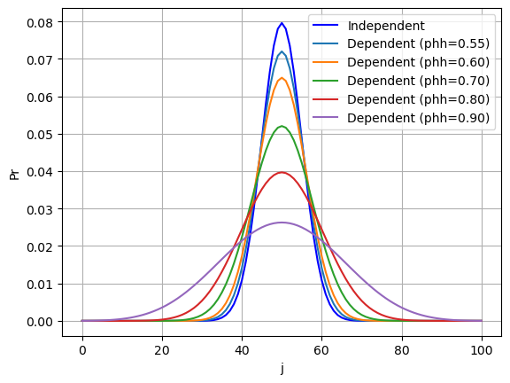
Figure 3: PDF of dependent vs independent binomial distributions. In all cases, the number of trials is K=100, simple trial success probability is P=0.5.
So the effect of positive serial correlation (\(P_{hh} > 0.5\)) tends to flatten out the probability distribution. Even with a slight preference for a hit to be followed by anothe (\(P_{hh} = 0.55\)), the bell curve already shows a notable drop in peak height.
6. Summary
This post covers a bit of the binomial distribution with dependent trials, based on the paper Ladd, Daniel W., 1975: An Algorithm for the Binomial Distribution with Dependent Trials.
Note that this doesn’t cover all of the paper’s content. For instance, the author talked about the determination of confidence intervals based on independent or dependent binomial models. This has potential implications on the comparison of distribution quantiles, a topic that has taken my interests recently. I might post a follow-up covering some of the rest of the interesting things in the paper.
Created: 2022-09-20 Tue 21:24


