Table of Contents
1. Overview
This is Part-3 of the series on building a YOLOv3 model from scratch.
Here is an overview of the series:
- Understand the YOLO model.
- Build the model backbone.
Load pre-trained weights: this post.
To verify the Darknet-53 model we built works as intended, we could load the pre-trained YOLOv3 weights and perform some inferences on some images.
- Get the tools ready.
- Training data preparation.
- Train the model.
2. Download the pre-trained weights
3. Write the weight-loading method
We are going to equip our Darknet53 model with a load_weights()
method that reads and loads the downloaded weights into the model
layers. So if you haven’t built the Darknet53 model, please go to
Part-2 of the series and get the model ready.
Below is the load_weights() method. Put it inside our Darknet53 class:
def load_weights(self, weight_file):
    '''Load pretrained weights'''

    def getSlice(w, cur, length):
        return torch.from_numpy(w[cur:cur+length]), cur+length

    def loadW(data, target):
        data = data.view_as(target)
        with torch.no_grad():
            target.copy_(data)
        return

    with open(weight_file, 'rb') as fin:
        # the 1st 5 values are header info
        # 1. major version number
        # 2. minor version number
        # 3. subversion number
        # 4,5. images seen by the network during training

        self.header_info = np.fromfile(fin, dtype=np.int32, count=5)
        self.seen = self.header_info[3]

        weights = np.fromfile(fin, dtype=np.float32)

    ptr = 0
    for layer in self.layers.values():
        if not isinstance(layer, ConvBNReLU):
            continue

        conv = layer.layers[0]

        if layer.bn:
            bn = layer.layers[1]
            # get the number of weights of bn layer
            num = bn.bias.numel()
            # load the weights
            bn_bias, ptr = getSlice(weights, ptr, num)
            bn_weight, ptr = getSlice(weights, ptr, num)
            bn_running_mean, ptr = getSlice(weights, ptr, num)
            bn_running_var, ptr = getSlice(weights, ptr, num)

            # cast the loaded weights into dims of module weights
            loadW(bn_bias, bn.bias)
            loadW(bn_weight, bn.weight)
            loadW(bn_running_mean, bn.running_mean)
            loadW(bn_running_var, bn.running_var)
        else:
            # number of conv biases
            num = conv.bias.numel()
            # load the weights
            conv_bias, ptr = getSlice(weights, ptr, num)
            loadW(conv_bias, conv.bias)

        # conv weights
        num = conv.weight.numel()
        conv_weight, ptr = getSlice(weights, ptr, num)
        loadW(conv_weight, conv.weight)

    assert len(weights) == ptr, 'Not all weight values loaded.'

    return
Some more explanations.
The pre-trained weights are saved in binary format, so we open it in
binary-reading (rb) mode:
with open(weight_file, 'rb') as fin:
The numpy.fromfile() function is used to read from the opened file
object.
The 1st 5 numbers are header information.
Starting from the 6th number are the model weights. We read them all
into a weights array:
self.header_info = np.fromfile(fin, dtype=np.int32, count=5)
weights = np.fromfile(fin, dtype=np.float32)
It is important to keep track of how many numbers we read from this big array. The exact number of weights needs to be read and fed into the correct places of the model layers, such that the trained weights can function as they were trained to do.
To help getting slices of numbers from the array, we create a
getSlice() helper function that cuts a slice starting from a pointed
location cur, with
length length. The function then shifts the pointer cur by length so
that it points to the next number to be read:
def getSlice(w, cur, length):
    return torch.from_numpy(w[cur:cur+length]), cur+length
Then we initialize the pointer ptr to point to the beginning of
the array weights, and enter into an iteration through the model
layers:
ptr = 0
for layer in self.layers.values():
    if not isinstance(layer, ConvBNReLU):
        continue
    conv = layer.layers[0]
Only convolutional layers have trainable weights, so we skip all other types of layers.
Recall that if the convolutional layer is followed by a batch
normalization, then the Conv2d module has no bias terms.
So we query the layer’s .bn attribute to see if it is case. If so,
we call bn.bias.numel() to get the number weights in the
BatchNorm2d module, slice out the weight numbers, and call a
loadW() helper function to feed the weights into the module:
if layer.bn:
    bn = layer.layers[1]
    # get the number of weights of bn layer
    num = bn.bias.numel()
    # load the weights
    bn_bias, ptr = getSlice(weights, ptr, num)
    bn_weight, ptr = getSlice(weights, ptr, num)
    bn_running_mean, ptr = getSlice(weights, ptr, num)
    bn_running_var, ptr = getSlice(weights, ptr, num)

    # cast the loaded weights into dims of module weights
    loadW(bn_bias, bn.bias)
    loadW(bn_weight, bn.weight)
    loadW(bn_running_mean, bn.running_mean)
    loadW(bn_running_var, bn.running_var)
If the convolutional layer has no batch normalization, then load a bias term:
else:
    # number of conv biases
    num = conv.bias.numel()
    # load the weights
    conv_bias, ptr = getSlice(weights, ptr, num)
    loadW(conv_bias, conv.bias)
Lastly, we slice out the weights for the convolutional kernel and feed
that into the Conv2d module:
# conv weights
num = conv.weight.numel()
conv_weight, ptr = getSlice(weights, ptr, num)
loadW(conv_weight, conv.weight)
Once the iteration through the network layers is finished, we should have a properly functioning YOLOv3. Let’s test that out.
4. Do some inferences using pre-trained weights
To test out whether the loaded weights function as expected, let’s get some images and run the model on them.
Below gives 4 sample images. Download them and save into the data
sub-folder of the YOLOv3_pytorch project folder.
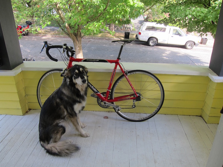
Figure 1: Sample image.
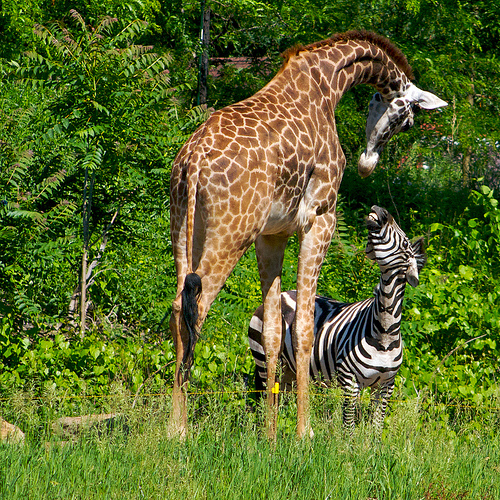
Figure 2: Sample image.
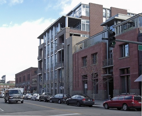
Figure 3: Sample image.
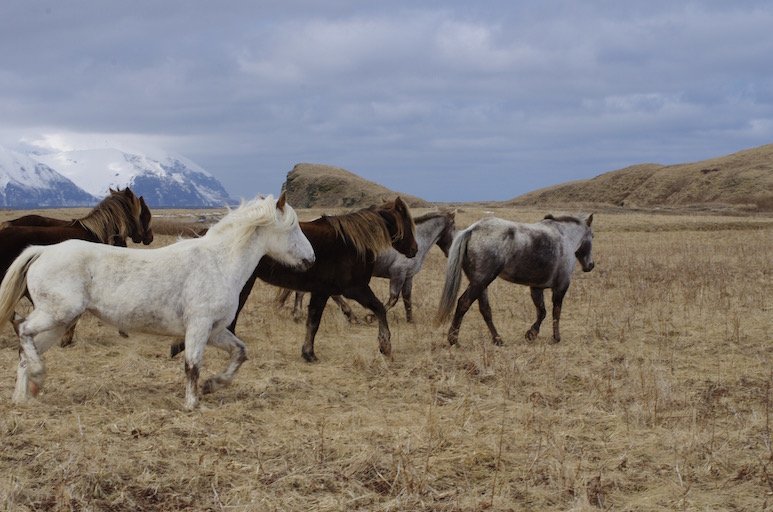
Figure 4: Sample image.
Then, download this coco.names_.txt file and save into the data sub-folder as
well. This is a list of 80 class names in the COCO detection
dataset.
Now create a predict_pretrained.py script in the YOLOv3_pytorch
folder, with these contents:
from __future__ import print_function
import os
import torch
from PIL import Image
from torchvision import transforms

from config import load_config
from model import Darknet53
from utils import read_coco_names, draw_predictions

#-------------Main---------------------------------
if __name__=='__main__':

    #--------------------Load model config--------------------
    CONFIG_FILE = './config/yolov3.cfg'
    net_config, module_list = load_config.parse_config(CONFIG_FILE)
    config = {'net': net_config}
    config['module_list'] = module_list
    config['width'] = 416
    config['height'] = 416
    config['n_classes'] = 80

    #-------------------Create model-------------------
    model = Darknet53(config)

    #-------------------Load weights-------------------
    weight_path = './yolov3.weights'
    model.load_weights(weight_path)

    #----------------Turn on eval model----------------
    model.eval()

    #------------Transform image to tensor------------
    trans = transforms.Compose([
        transforms.Resize([config['width'], config['height']]),
        transforms.ToTensor()])

    #--------------------Load data classes--------------------
    coco_name_file = './data/coco.names_.txt'
    class2id, id2class = read_coco_names(coco_name_file)
    print('\nclass2id:')
    print(class2id)

    #--------------Load some test images--------------
    data_folder = './data'
    img_files = os.listdir(data_folder)

    for fii in img_files:
        if os.path.splitext(fii)[1] != '.jpg':
            continue

        img_fileii = os.path.join(data_folder, fii)
        print('\nReading image file:', img_fileii)
        imgii = Image.open(img_fileii)

        # transform image to tensor
        img_tensor = trans(imgii).unsqueeze(0)

        # make prediction
        with torch.no_grad():
            y = model(img_tensor)

        print('y.shape:', y.shape)
        y = y.detach().cpu().numpy().squeeze()
        print('y.shape:', y.shape)

        # filter by confidence
        y_conf = y[:, 4]
        idx = y_conf >= 0.96
        y_filtered = y[idx]

        if len(y_filtered) > 0:
            # draw predictions
            fig, ax = draw_predictions(imgii, model.width, model.height, y_filtered, id2class)
            fig.show()
The code is fairly self-explanatory. Just note that we are filtering the predictions by selecting those with confidence scores >= 0.96. This is only a temporary solution. Typically we will need to follow it up by a Non-maximum suppression. We will cover that in a later post.
To make it work, we also need to 2 utility functions:
read_coco_names(): read the class names in thecoco.names_.txtfile, and create 2dicts: one for mapping the class names to integer ids, and the other does the opposite.draw_predictions(): draw the image and bounding boxes of detections on top of it.
I put these 2 functions in a utils.py file in the YOLOv3_pytorch
folder.
Here is the read_coco_names() function:
def read_coco_names(file_path):

    with open(file_path, 'r') as fin:
        names = fin.readlines()

    class2id = dict([(xx.strip(), ii) for (xx, ii) in zip(names, range(len(names)))])
    id2class = dict([(vv,kk) for (kk,vv) in class2id.items()])

    return class2id, id2class
Fairly straightforward. Now the draw_predictions() function:
import numpy as np
import matplotlib.pyplot as plt
from matplotlib import patches

def draw_predictions(img, input_w, input_h, pred, id2class):
    '''Draw object detection predictions

    Args:
        img (PIL.Image): image to detect objects from.
        input_w (int): width of image as input to model.
        input_h (int): height of image as input to model.
        pred (ndarray): n x m ndarray, n is number of selected detections.
            m = 5 + n_classes.
        id2class (dict): dict containing id-to-class name key-value pairs.
    '''

    figure = plt.figure(figsize=(12,10), dpi=100)
    ax = figure.add_subplot(1,1,1)
    ax.imshow(img)
    img_w, img_h = img.size

    for pii in pred:

        boxii = pii[:4]  # x, y, w, h
        # scale to original image size
        boxii[[0, 2]] *= img_w / input_w
        boxii[[1, 3]] *= img_h / input_h
        # get top-left corner
        xc, yc, w, h = boxii
        x1 = xc - w/2
        y1 = yc - h/2
        # create bbox
        recii = patches.Rectangle((x1, y1), w, h, facecolor='none', edgecolor='w')
        ax.add_patch(recii)
        # prepare label
        confii = pii[4]
        clsii = np.argmax(pii[5:])
        labelii = '%s %.2f' %(id2class[clsii], confii)
        ax.text(x1, y1, labelii, ha='left', va='bottom', bbox={'color': 'c', 'alpha': 0.6})

    return figure, ax
I’m using matplotlib to do the drawings. Feel free to use opencv
if you like.
5. Sample results
Below are the detection results corresponding to the sample images shown above:
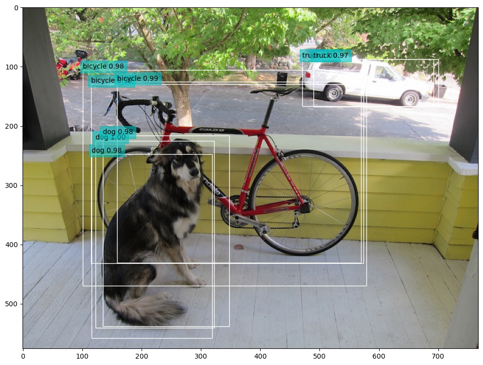
Figure 5: Sample image detection result.
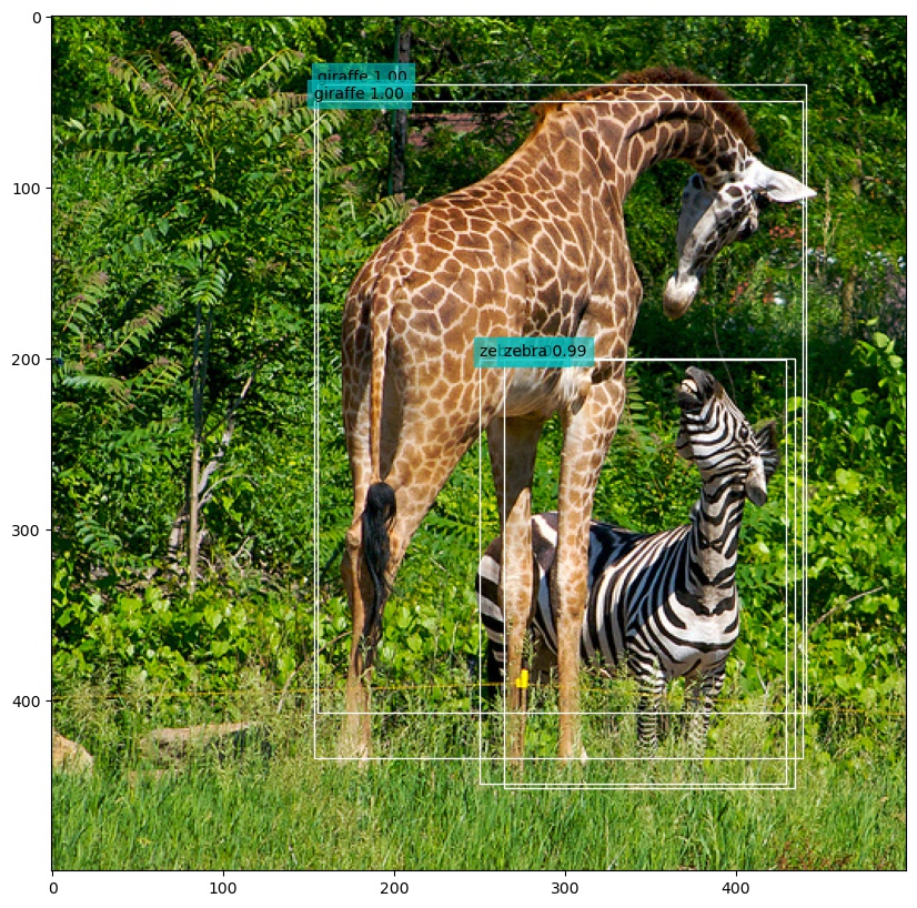
Figure 6: Sample image detection result.
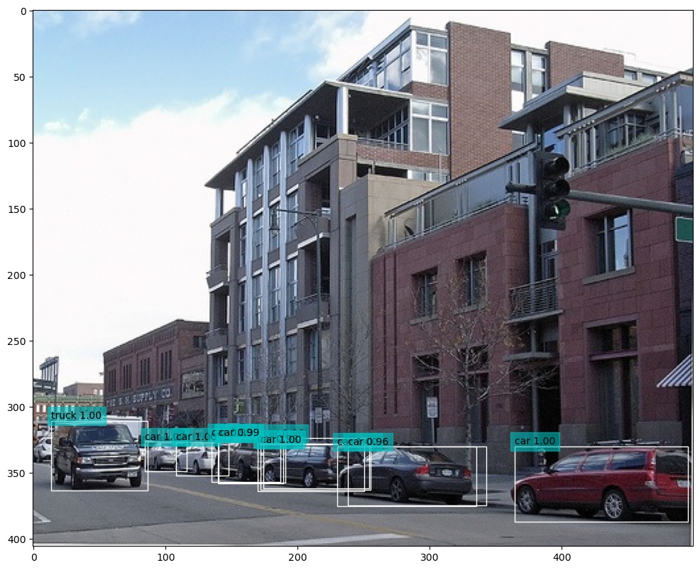
Figure 7: Sample image detection result.
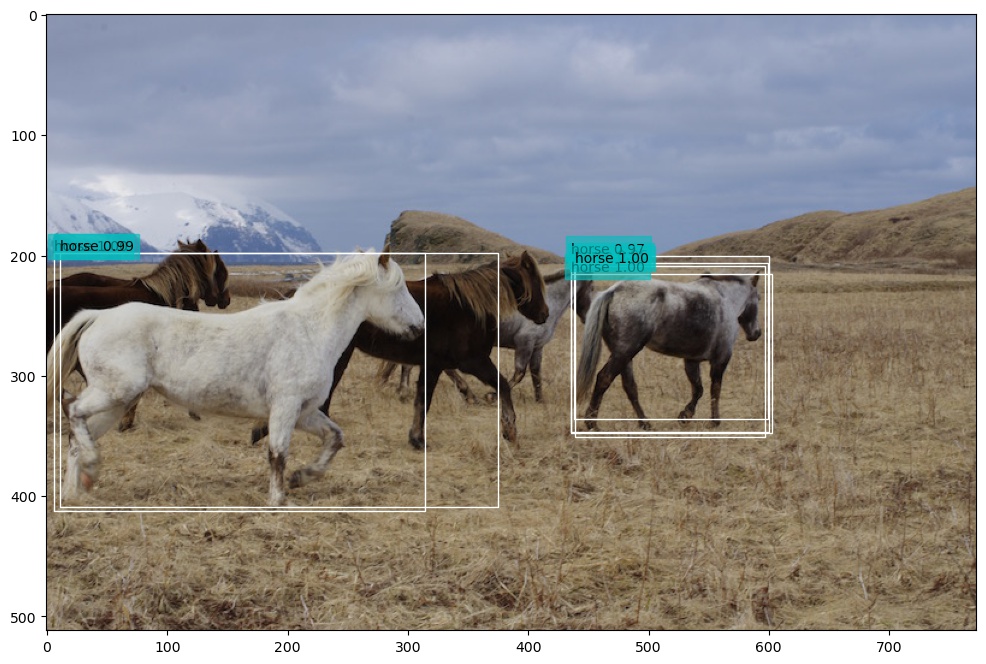
Figure 8: Sample image detection result.
The results are not bad. The model correctly detected with high confidence the objects and correctly classified them.
But there are many overlapping detections. This could be solved by running a Non-maximum suppression filtering. We will get to that in the next post. So stay tuned.
Created: 2022-06-22 Wed 22:38


