What is "Silhouette value"?
To quote the definition from wikipedia:
Silhouette refers to a method of interpretation and validation of
consistency within clusters of data.  …  The silhouette value is a
measure of how similar an object is to its own cluster (cohesion)
compared to other clusters (separation). The silhouette ranges from −1
to +1, where a high value indicates that the object is well matched to
its own cluster and poorly matched to neighboring clusters. If most
objects have a high value, then the clustering configuration is
appropriate. If many points have a low or negative value, then the
clustering configuration may have too many or too few clusters.
Therefore, silhouette value is a measure of the effectiveness of the clustering analysis, and can be used to help determine a more desirable cluster number.
A typical visual representation of the silhouette values can be seen in this example given by scikit-learn:
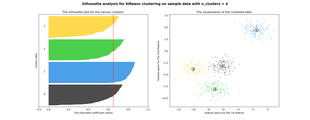
In this case, the data to be clustered are plotted out as a scatter
plot on the right, and the clustering is performed using a K-means
clustering, with parameter k=4. The resultant 4 clusters are labeled
out in the scatter plot, with their respective members color
coded. Silhouette value for each sample member is plotted in the
graph on the left, with matching colors denoting the membership. The
silhouette values have been sorted such that in each cluster, the
member silhouette values form a "knife-like" shape. A more effective
clustering would produce higher silhouette values in all clusters,
therefore blunter knives, and vice verse.
Mathematical definition
[latexpage]
The Silhouette value $s(i)$ of a sample $i$ is defined as:
\[
s(i) = \begin{cases}
\frac{b(i) – a(i)}{max \{ a(i), b(i)\} } & \text{ if } |C_i| >1 \\
0 & \text{ if } |C_i| = 1
\end{cases}
\]
where $a(i)$ is the mean intra-cluster distance of sample $i$ to
other members in the same cluster $C_i$:
\[
a(i) = \frac{1}{(|C_i| – 1)} \sum_{j \in C_i, i \neq j} d(i,j)
\]
$d(i,j)$ is the distance measure, which can be taken as Euclidean
distance, or a city-block distance, or whatever distance measure.
$b(i)$ is the mean inter-cluster distance of sample $i$ to its nearest
neighbor cluster $C_k$:
\[
b(i) = \underset{k \neq i}{min}
\frac{1}{|C_k|} \sum_{j \in Ck} d(i,j)
\]
A Python implementation
There is nothing complex in the formulae, involving only simple math
calculations, and there is also a built-in function to compute the
sample Silhouette values in the
scikit-learn package.
Here, we only give a "custom"
Python implementation, using the scipy.spatial.distance_matrix to
compute the distances (d(i,j)).
Code below:
def sampleSilhouette(data, labels, norm=2, cluster=None):
    '''Compute Silhouette value for each sample

    Args:
        data (ndarray): Nxk ndarray, samples. N is the number of records, k
            the number of features.
        labels (ndarray): 1darray with length N, the cluster number for each
            sample in <data>.
    Keyword Args:
        norm (int): p-norm. Default to 2.
        cluster (int or None): if None, compute Silhouette values for all
            samples and the return value is Nx1. If int, only return Silhouette
            values of samples belonging to cluster labelled <cluster>.
    Returns:
        results (ndarray): nx1 ndarray of the Silhouette values.
            If <cluster> is None, N=n. If <cluster>
            is an int, n is the number of cluster members in cluster <cluster>.

    Definition of Silhouette value:

        s(i) = (b(i) - a(i))/max{a(i), b(i)}    if |Ci| > 1
             = 0                                  if |Ci| = 1

        a(i) is the mean intra-cluster distance of sample i to other members
        in the same cluster Ci:

            a(i) = 1/(|Ci| - 1) \sum_{j \in Ci, i \neq j} d(i,j)

        b(i) is the mean inter-cluster distance of sample i to its nearest
        neighbor cluster Ck:

            b(i) = min_{k \neq i} 1/|Ck| \sum_{j \in Ck} d(i,j)
    '''

    from scipy.spatial import distance_matrix

    # all pair-wise distances
    dists=distance_matrix(data, data, p=norm)

    clusters=np.unique(labels)
    nclusters=len(clusters)
    results=np.zeros(len(data))

    # distance to members in cluster i
    dist2clusteri=[]
    members=[]

    for ii,cii in enumerate(clusters):
        membersii=np.where(labels==cii)[0]
        sumii=np.sum(dists[membersii], axis=0)
        dist2clusteri.append(sumii)
        members.append(membersii)

    if cluster is None:
        loop_clusters=clusters
        sel_idx=slice(None)
    else:
        if not cluster in clusters:
            raise Exception("Target cluster not found in <labels>.")

        # compute only specified cluster members
        loop_clusters=[cluster,]
        sel_idx=members[list(clusters).index(cluster)]

    #--------------Loop through clusters--------------
    for ii,cii in enumerate(clusters):
        if cii not in loop_clusters:
            continue

        membersii=members[ii]
        if len(membersii)<=1:
            sii=0
        else:
            # mean intra-cluster dist
            aii=dist2clusteri[ii][membersii]/float(len(membersii)-1)
            # mean inter-cluster dist to other clusters
            biis=[]
            for jj in range(nclusters):
                if jj==ii:
                    continue
                membersjj=members[jj]
                bij=dist2clusteri[jj]/float(len(membersjj))
                bij=bij[membersii]
                biis.append(bij)

            biis=np.array(biis)
            bii=np.min(biis, axis=0)
            sii=(bii-aii)/np.max(np.c_[aii, bii], axis=1)

        results[membersii]=sii

    # select desired cluster members
    results=results[sel_idx]

    return results
A few points to note
inter-point distances
[latexpage]
The silhouette value is all about inter-point distances in a multi-dimensional space. For a clustering of $N$ points, there are $N\times(N-1)$ non-trivial inter-point distance pairs, if the distance measure is not directed (the distance from point $i$ to $j$ is the same as that from $j$ to $i$). When computing the silhouette value for sample $i$, it is using the distance from sample $i$ to all the other samples $j, j \neq i$. Therefore, it would be more efficient to get all the pair-wise distances first, rather than re-compute them as we loop through the samples.
To get all the pair-wise distances in one go, we used the
scipy.spatial.distance_matrix() function:
dists=distance_matrix(data, data, p=norm)
dists is a $N \times N$ symmetrical matrix, with 0s at its
diagonal line. The distance between sample $i$ and $j$ is at
dists[i,j].
For Euclidean distance, one would use (p=2) argument for the Minkowski
2-norm distance measure. (Internally, distance_matrix() is calling
scipy.spatial.minkowski_distance() for the computation.)
For other distance measures, one could use
scipy.spatial.distance.cdist() function. For instance:
dists=cdist(data, data, metric='cityblock')
for a city-block (a.k.a Manhattan) distance,
or
dists=cdist(data, data, metric='wminkowski', p=2, w=W)
for a weighted Euclidean distance with weights provided in W.
Distance to/from members in a cluster
[latexpage]
Since all the $N \times (N-1)$ pairs of distances have been computed in one go, all we need to do next is to get the correct distances to compute the average intra-cluster distance $a(i)$ and inter-cluster distance $b(i)$.
The cluster membership information is provided in the argument labels, which is a $N \times 1$ vector denoting the membership for each sample. Indices for the members in cluster cii is obtained by:
membersii=np.where(labels==cii)[0]
Therefore, distances to these members can be obtained from the distance matrix using:
dists[membersii]
Note that is also the distances from these members, to all other samples, since the distance matrix is symmetrical.
Then, the average intra-cluster distance in cluster cii, for each
member in the same cluster is:
aii = np.sum(dists[membersii], axis=0)[membersii]/(len(membersii)-1)
The average inter-cluster distance $b(i)$ is defined on the nearest neighbor cluster, therefore, we will need to loop through all other clusters, compute the inter-cluster distance, and get the minimum. For each cluster neighbor, the average distance is:
bij = np.sum(dists[membersjj], axis=0)[membersii]/len(membersjj)
After getting all $bij$s, the minimum is simply:
bii = np.min(biis, axis=0)
Note that in finding the aiis and biis, we called
np.sum(dists[membersii], axis=0) multiple times. So it would be
better to compute these before hand, and only query them when needed,
to avoid repeated computations. This is done in these lines:
    dist2clusteri=[]
    members=[]

    for ii,cii in enumerate(clusters):
        membersii=np.where(labels==cii)[0]
        sumii=np.sum(dists[membersii], axis=0)
        dist2clusteri.append(sumii)
        members.append(membersii)
Vectorize computations
Also note that we are not performing a loop through the N samples,
but only a loop through the clusters. This is because much of the
computations are vectorized, and all the distances have been computed
in one go. As Python is slow for nested loops, it can be crucial to
vectorize as much computations as possible, by using, for instance,
matrix computations, or smart indexing. In a future post, I will share
an implementation of the Histogram of Orientated Gradients (HOG)
feature extraction algorithm, which can be used in pedestrian
detection applications. Using the smart indexing approach, the
vectorized HOG implementation is able to achieve 2-3 times speed up
compared with the scikit-image implementation using cython.


