The goal
This post will share some basic knowledge of an artificial neural
network and how to create one from scratch using only numpy. As a
concrete example, we will build a classification network and use it to
classify hand-written digits from the MNIST dataset.
We will start by introducing the general idea and structure of the
network, and the mathematical notations. The computations involved
inside the network will be introduced by first showing the math
equations, followed with the numpy implementations in the 2nd part
of the post. If a
particular step can be optimized, for instance, by vectoring the
computations, these will be covered as well. In the end, the network is
trained on the training dataset of MNIST, and its performance
evaluated using MNIST’s test data. The final, complete code is given at
this simple-nn Github repo.
Computations in the network and notations
Layers in the network
The network we will be building consists of 5 layers:
1. input layer (layer-0): this is the layer that feeds the input data into the network.
The number of neurons (or units) in the input layer should be the same as the size of the input data. In this particular case, the input data are images of MNIST hand-written digits. Each image is 28 pixels x 28 pixels in size, and we flatten the image into a single array of length 28 x 28 = 784. Therefore, the input layer has 784 neurons.
We denote the size of layer \(l\) as \(s_l\). Therefore, \(s_0=784\).
Note that we are indexing the layer number starting from index 0, i.e. the 1st layer has index 0, 2nd has index 1, and so on. This is mostly arbitrary. In some places people label the input layer as layer-1. Using 0-based indexing makes it only slightly convenient to work with Python whose array indices also start from 0.
2. 3 hidden layers (layer-1, layer-2 and layer-3): these layers have sizes:
- layer-1: 200 neurons, \(s_1=200\).
- layer-2: 100 neurons, \(s_2=100\).
- layer-3: 50 neurons, \(s_3=50\).
NOTE that these are also arbitrary choices. We are not going to compare different design choices in this post. It is totally possible that a simpler or different design would work just as well or even better.
3. output layer (layer-4): this is the layer that outputs the final result of the network. The final result is often termed as the prediction of the model. It is conventional to label the prediction as \(\hat{y}\) (or \(\mathbf{\hat{y}}\)).
For the task of recognizing hand-written digits from images, it is a multi-class classification problem. There are a total of 10 classes in the problem, corresponding to digits from 0 to 9. For such kind of tasks, it is common to formulate the prediction using the so-called one-hot encoding. For instance, the label for digit 0 is defined as
\[
[1, 0, 0, 0, 0, 0, 0, 0, 0, 0]
\]
that for digit 1 as
\[
[0, 1, 0, 0, 0, 0, 0, 0, 0, 0]
\]
and similarly, digit 5 is encoded as:
\[
[0, 0, 0, 0, 0, 5, 0, 0, 0, 0]
\]
More generally, the class i in a K-class classification task is represented by a K-length vector whose i-th element is 1, and all other places are 0s.
Therefore, the output layer has 10 neurons: \(s_{4}=10\).
To summarize this section:
- The network has multiple layers, 1 input layer, 1 output layer, and all other layers in-between are called hidden layers.
- The number of layers in the network is denoted \(L\). The number of neurons/units in layer \(l\) is denoted as \(s_l\). In this case, \(L=5\), \(s_0 = 784\), \(s_1 = 200\), \(s_2 = 100\), \(s_3 = 50\), and \(s_4 = 10\). The input and output layer sizes are determined by the specific problem to be solved, and hidden layer sizes are design choices.
- one-hot encoding is used for the digit classification task.
Computations happening inside the network – the forward propagation
Information gets passed from the input layer (layer-0) to the 1st hidden layer (layer-1), then to all subsequent layers, one layer at a time.
From layer-0 to layer-1, each neuron \(j\) in layer-0 is connected to each neuron \(i\) in layer-1. Therefore, there are a total of \(s_1 \times s_0 = 200 \times 784 = 157200\) connections. That is quite a number of connections, that is why such models are also called dense networks.
Similarly, from layer-1 to layer-2, there are \(s_2 \times s_1 = 100 \times 200 = 20000\) connections.
More generally, from layer \(l\) to layer \(l+1\), the number of connections is \(s_{l+1} \times s_{l}\).
What happens along these connections is a linear operation. More specifically, suppose that the neuron \(i\) at layer \(l\) is sending a value to neuron \(j\) in the next layer. The value sent is termed \(a_{i}^{(l)}\), where \(a\) stands for activation. The linear operation is
\[
z_{j}^{(l+1)} = a_{i}^{(l)} \theta_{j,i}^{(l+1)} + b_{j}^{(l+1)}
\]
where:
- \(\theta_{j,i}^{(l+1)}\) is a weight that is associated with the connection between these 2 neurons. The weight is multiplied with the input activation value \(a_{i}^{(l)}\).
- \(b_{j}^{(l+1)}\) is a bias term added onto the product.
- \(z_{j}^{(l+1)}\) is the result of the linear operation. Intuitively, this is what a next layer neuron receives from its upstream input.
After getting \(z_{j}^{(l+1)}\), the neuron gets “activated”, and sends out an “activation” to its next layer. This “activation” is mathematically achieved by an activation function:
\[
a_{j}^{(l+1)} = g(z_{j}^{(l+1)})
\]
where \(g()\) is the activation function, which is typically a non-linear function, for instance, a logistic function (a.k.a sigmoid function):
\[
g(z) = \frac{1}{1 + e^{-z}}
\]
Therefore, the processes happening in from layer \(l\) to \(l+1\) are:
\[
\left\{\begin{matrix}
z_{j}^{(l+1)} =& a_{i}^{(l)} \theta_{j,i}^{(l+1)} + b_{j}^{(l+1)} \\
a_{j}^{(l+1)} =& g(z_{j}^{(l+1)})
\end{matrix}\right.
\]
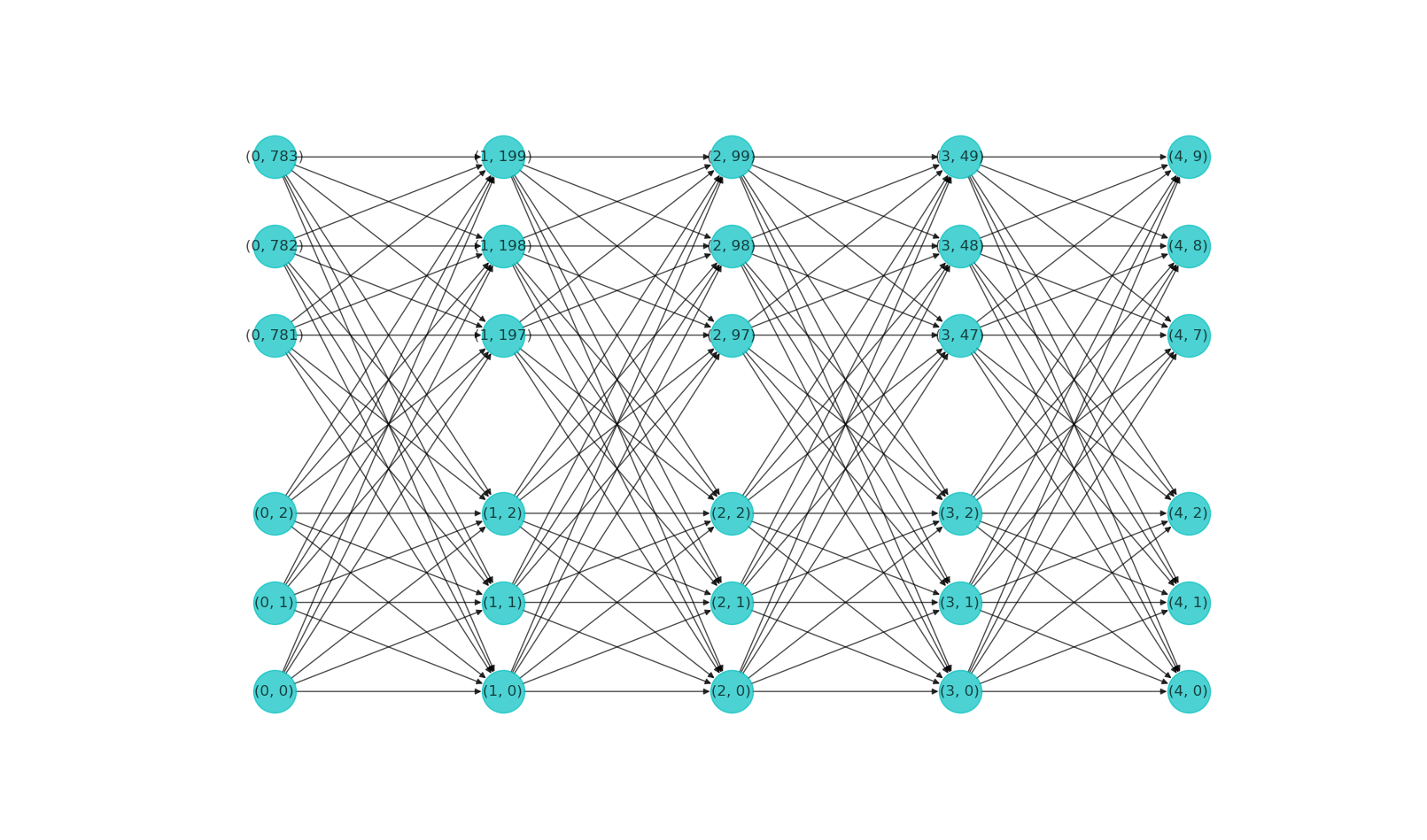
Then the similar process is repeated from layer \(l+1\) to \(l+2\), and so on, till the very last layer in the network. This process is called forward propagation. See figure below for an illustration.
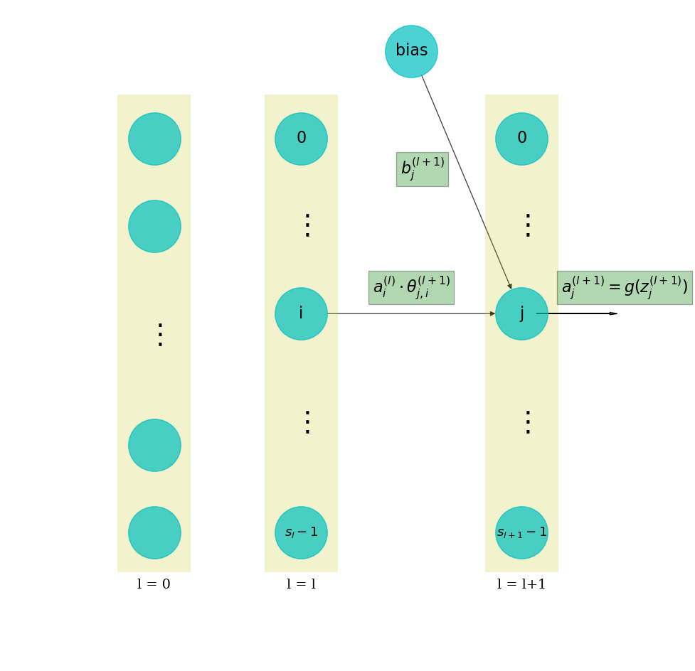
NOTE that for the 1st layer, \(a^{(0)}\) is just the input data in layer-0. For the last layer, \(a^{(L-1)}\) is the model prediction.
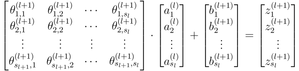
Recall that there are \(s_{l+1} \times s_{l}\) number of connections between layer \(l\) and \(l+1\), meaning \(s_{l+1} \times s_{l}\) number of linear operations. All these could be neatly represented using matrix-vector notations as below:
Or more compactly:
\[
\mathbf{\Theta}^{(l+1)} \cdot \mathbf{a}^{(l)} + \mathbf{b}^{(l+1)} = \mathbf{z}^{(l+1)}
\]
where:
- \(\mathbf{\Theta}^{(l+1)}\) is the weight matrix that maps data from layer l to layer l+1. It has a dimension of \((s_{l+1} \times s_l)\). The element, \(\theta_{j,i}^{(l+1)}\) is the weight associated with the link from neuron \(j\) in layer \(l\), to neuron \(i\) in layer \(l+1\).
- \(\mathbf{a}^{(l)}\) is the vector of activations from layer \(l\), with dimension \((s_l \times 1)\).
- \(\mathbf{b}^{(l+1)}\) is the vector of biases added to layer \(l+1\), with dimension \((s_{l+1} \times 1)\).
- \(\mathbf{z}^{(l+1)}\) is the weighted sum in layer \(l+1\), with dimension \((s_{l+1} \times 1)\).
The activation process is simply:
\[
\mathbf{a}^{(l+1)} = g(\mathbf{z}^{(l+1)})
\]
where \(\mathbf{a}^{(l+1)}\) is the vector of activations in layer \(l+1\), with dimension \((s_{l+1} \times 1)\).
To summarize this section:
- Information passes from the input layer through hidden layer(s) to the output layer, a process called forward propagation.
- Between 2 consecutive layers \(l\) and \(l+1\), data get passed in a linear operation: \(\mathbf{\Theta}^{(l+1)} \cdot \mathbf{a}^{(l)} + \mathbf{b}^{(l+1)} = \mathbf{z}^{(l+1)}\).
- A non-linear activation function is used to transform the weighted sum of a layer to its output: \(\mathbf{a}^{(l+1)} = g(\mathbf{z}^{(l+1)})\).
- \(\mathbf{a}^{(0)}\) is the input data, \(\mathbf{a}^{(L-1)}\) is the model prediction.
NOTE that some materials may use a slightly different formula for the linear operation:
\[
\mathbf{\Theta}^{(l)} \cdot \mathbf{a}^{(l)} + \mathbf{b}^{(l+1)} =
\mathbf{z}^{(l+1)}
\]
This is because \(\mathbf{\Theta}^{(l)}\) is used to denote the mapping from layer \(l\) to \(l+1\), while we used \(\mathbf{\Theta}^{(l+1)}\) for this. So it is a purely a notational difference, and the underlying processes are identical. This notation is chosen because I found it slightly more intuitive to associate a layer with the weights that pass data to the layer. This minor advantage may become more obvious when dealing with convolution neural networks where different types of layers are concatenated.
ALSO NOTE that for the multi-class classification problem, the output layer needs to use the softmax activation function, which is the generalization of logistic to multi-dimensional data. The softmax function for a vector \(x = \{x_0, x_1, \cdots, x_{n-1}\}\) is defined as:
\[
\sigma(x)_j = \frac{e^{x_j}}{\sum_i e^{x_i}}
\]
Computations happening inside the network – the cost function
The cost function is a function that computes the cost J, which is a scalar value that measures the goodness-of-fit of the model. A smaller cost means a better fit of the model prediction. There are multiple ways to define a cost, for different types of problems. For the multi-class classification problem, a typical choice is the cross-entropy cost function. The cost contributed by single record is:
\[
J_i = J(\mathbf{\hat{y}}_i, \mathbf{y}_i) = – \mathbf{y}_i \cdot log(\mathbf{\hat{y}}_i)
\]
The cost of all the training samples is just the average over all \(m\) samples:
\[
J = \frac{1}{m} \sum_i^m J_i = – \frac{1}{m} \sum_i^m [\mathbf{y}_i \cdot log(\mathbf{\hat{y}}_i)]
\]
For good measure, let’s also add the regularization term:
\[
J = – \frac{1}{m} \sum_i^m [\mathbf{y}_i
\cdot log(\mathbf{\hat{y}}_i)] + \frac{\lambda}{m}
\sum_{l=1}^{L-1} \sum_{i=1}^{s_l} \sum_{j=1}^{s_{l+1}} {\theta_{j,i}^{(l)}}^2
\]
where \(\lambda\) is the regularization parameter. Note that the nested summations in the above equation are just summing up all (squared) weights in all layers, and biases are not included in the regularization term.
Computations happening inside the network – the backward propagation
Training of a neural network classifier is a supervised learning process, where the model makes a prediction, which is compared with the true value (a.k.a label), and a correction to the model is made accordingly, if needed. The prediction is achieved using the forward propagation, and the correction is done in a process called back-propagation. This forward-backward propagation process is repeated multiple times until a desired skill level of the model is achieved.
Intuitively, the back-propagation finds the error made by the model by comparing the final prediction \(\mathbf{\hat{y}}\) with the label \(\mathbf{y}\): \(\mathbf{\delta} \equiv \mathbf{\hat{y}} – \mathbf{y}\). This error is then propagated backwards from the output layer to hidden layer(s).
This backward error propagation is done because we need to compute the gradients of the weights and biases. Recall that training a model is the same process of adjusting its parameters such that the predictions fit the expected values better. For a neural network, its parameters are the weight matrices and bias vectors associated with the layers.
The gradients of weights are formally defined as \(\frac{\partial J}{\partial \mathbf{\Theta}}\), and gradients of biases are defined as \(\frac{\partial J}{\partial \mathbf{b}}\).
Next we give (without proof) the 2 formulae describing the back-propagation process. More details of the derivation will be covered in a separate post.
Starting from the output layer. The error of the output layer is simply:
\[
\mathbf{\delta}^{(L-1)} = \mathbf{\hat{y}} – \mathbf{y}
\]
(1)
From layer \(L-1\) backwards, the error that gets propagated from layer \(l\) to \(l-1\) is:
\[
\begin{equation}
\mathbf{\delta}^{(l-1)} = {\mathbf{\Theta}^{(l)}}^T \cdot
\mathbf{\delta}^{(l)} \odot g'(\mathbf{z}^{(l-1)})
\end{equation}
\]
(2)
where:
- \(\mathbf{\delta}^{(l)}\) is the error of layer \(l\). More formally, this is defined as \(\mathbf{\delta}^{(l)} \equiv \frac{\partial J}{\partial \mathbf{z}^{(l)}}\).
- \(\odot\) is the Hadamard product, a.k.a element-wise product.
- \(g'()\) is the derivative of the activation function.
One can give a quick check of the dimensions in each term:
- \(\mathbf{\delta}^{(l-1)}\): same as \(\mathbf{a}^{(l-1)}\): \((s_{l-1} \times 1)\).
- \({\mathbf{\Theta}^{(l)}}^T\): \((s_{l-1} \times s_l)\).
- \(\mathbf{\delta}^{(l)}\): same as \(\mathbf{a}^{(l)}\): \((s_l \times 1)\).
- \(g'(\mathbf{z}^{(l-1)})\): same as \(\mathbf{z}^{(l-1)}\): \((s_{l-1} \times 1)\).
It is trivial to see that dimensions on both side match.
The 2nd formula involves the computation of gradients in each layer:
\[
\left\{\begin{matrix}
\frac{\partial J}{\partial \mathbf{\Theta}^{(l)}} = & \mathbf{\delta}^{(l)} \cdot {\mathbf{a}^{(l-1)}}^{T} \\
\frac{\partial J}{\partial \mathbf{b}^{(l)}} = & \mathbf{\delta}^{(l)}
\end{matrix}\right.
\]
(3)
where:
- \(\frac{\partial J}{\partial \mathbf{\Theta}^{(l)}}\) is the gradients of cost function wrt the weights associated with layer \(l\).
- \(\frac{\partial J}{\partial \mathbf{b}^{(l)}}\) is the gradients of cost function wrt the biases associated with layer \(l\).
These gradients can be used to update the parameters using, for instance, a gradient descent scheme.
Notice that \(\mathbf{\Theta}^{(l)}\) is the weights mapping from layer \(l-1\) to \(l\). Therefore, a mnemonic for the above equation is:
gradients of the weights (\(\partial J/ \partial \Theta\)) is the product of the inputs into the weights (\(a^{(l-1)}\)) and the error out from the weights (\(\delta^{(l)}\)).
Gradient descent update
We will be using the basic gradient descent update scheme for this one. There are various derivations aimed at improving the convergence process, and some of them will be introduced in a later post.
The formula for updating the layer weights is:
\[
\mathbf{\Theta} := \mathbf{\Theta} – \frac{\alpha}{m} \sum_i^m \frac{\partial J_i}{\partial
\mathbf{\Theta}} – \frac{\alpha \lambda}{m} \mathbf{\Theta}
\]
The formula for updating the layer biases is:
\[
\mathbf{b} := \mathbf{b} – \frac{\alpha}{m} \sum_i^m \frac{\partial J_i}{\partial \mathbf{b}}
\]
where \(\alpha\) is the learning rate, \(\lambda\) the regularization parameter.
Recap on the notations
It might be worthwhile giving a recap on the notations introduced so far:
- \(L\): number of layers in a neural network.
- \(l\): index of a layer. \(l = 0, 1, \cdots, L-1\).
- \(s_l\): number of neurons/units in layer \(l\).
- \(\theta_{j,i}^{(l)}\): weight that maps from neuron \(i\) in layer \(l-1\) to neuron \(j\) in layer \(l\).
- \(b_{j}^{(l)}\): bias added onto neuron \(j\) in layer \(l\).
- \(z_{j}^{(l)}\): weighted sum of neuron \(j\) in layer \(l\).
- \(a_{j}^{(l)}\): activation of neuron \(j\) in layer \(l\).
- \( \mathbf{\Theta}^{(l)} \) : weight matrix that maps from layer \(l-1\) to layer \(l\).
- \(\mathbf{b}^{(l)}\): bias vector added onto layer \(l\).
- \(\mathbf{z}^{(l)}\): weighted sum vector of layer \(l\).
- \(\mathbf{a}^{(l)}\): activation vector of layer \(l\).
- \(g()\): activation function.
- \(\mathbf{\hat{y}}\): vector of model prediction.
- \(\mathbf{y}\): vector of label.
- \(\mathbf{\delta}^{(l)}\): vector of error in layer \(l\).
- \(J\): cost function value.
- \(\odot\): Hadamard product, a.k.a element-wise product.
numpy implementation
This section introduces the Python implementation of the above computations. The results will be used as building blocks of the final neural network.
Softmax function
The softmax function can be easily implemented in numpy as:
def softmax(x):
	return np.exp(x) / np.sum(np.exp(x))
Alternatively, there is also a function in scipy: scipy.special.softmax.
Logistic function and its derivative
def logistic(x):
	return 1 / (1 + np.exp(-x))
Alternatively, there is also a function in scipy: scipy.special.expit.
The derivative of logistic is:
def dlogistic(x):
	'''Derivative of the logistic function'''
	return np.exp(-x)/(1 + np.exp(-x))**2
Cross-entropy function
def crossEntropy(yhat, y):
	'''Cross entropy cost function '''
	eps = 1e-10
	yhat = np.clip(yhat, eps, 1-eps)
	return - np.nansum(y*np.log(yhat))
This is basically a literal translation of the mathematical equation
into Python language, with the only exception that a small value
(eps) is added to the yhat term to avoid infinities from the
logarithm function when yhat = 0, and the same eps is subtracted from 1 just to
make it symmetrical.
Cost function
The cost consists of 2 parts:
- errors of the model contributed by training samples. This is
computed in a
sampleCost()function. - penalties by the regularization term. This is computed in a
regularizationCost()function.
def samplecost(self, yhat, y):
	'''cost of a single training sample/batch

	args:
	yhat (ndarray): prediction in shape (n, m). m is the number of
		final output units, n is the number of records.
	y (ndarray): label in shape (n, m).
	returns:
	cost (float): summed cost.
	'''
	return self.cost_func(yhat, y)

def regulizationcost(self):
	'''cost from the regularization term

	defined as the summed squared weights in all layers, not including
	biases.
	'''
	j = 0
	for ll in range(1, self.n_layers):
	j = j+np.sum(self.thetas[ll]**2)
	return j
Here, self.cost_func is just the crossEntropy() function
defined above. The latter is passed in to the constructor of the class
such that it is more flexible to switch to a different cost function
definition should one decides to.
Forward propagation
The forward propagation consists of 2 equations, each corresponding to basically 1 line of code:
z = np.dot(a, thetas.T) + b
a = activation(z)
This should be fairly self-explanatory. However, in practice, some extra house-keeping and structuring are needed. The full function can be implemented as follows:
def feedForward(self, x):
	'''Forward pass

	Args:
	x (ndarray): input data with shape (n, f). f is the number of input units,
		n is the number of records.
	Returns:
	weight_sums (dict): keys: layer indices starting from 0 for
		the input layer to N-1 for the last layer. Values:
		weighted sums of each layer:

		z^{(l+1)} = a^{(l)} \cdot \theta^{(l+1)}^{T} + b^{(l+1)}

		where:
		z^{(l+1)}: weighted sum in layer l+1.
		a^{(l)}: activation in layer l.
		\theta^{(l+1)}: weights that map from layer l to l+1.
		b^{(l+1)}: biases added to layer l+1.

		The value for key=0 is the same as input <x>.
	activations (dict): keys: layer indices starting from 0 for
		the input layer to N-1 for the last layer. Values:
		activations in each layer. See above.
	'''
	x = self.force2D(x)
	activations = {0: x}
	weight_sums = {0: x}
	a1 = x
	for ii in range(1, self.n_layers):
	bii = self.biases[ii]
	zii = np.dot(a1, self.thetas[ii].T)+bii
	if ii == self.n_layers-1:
		aii = self.af_last(zii)
	else:
		aii = self.af(zii)
	activations[ii] = aii
	weight_sums[ii] = zii
	a1 = aii

	return weight_sums, activations
Firstly, we are going to assume (and therefore require) that the input
data records are arranged in rows. That is to say, the input variable x is
an ndarray of shape (m, f), where m being the number of records,
and f the number of features (in the case of MNIST data, f = 784).
To enforce this rule on a single data record with a shape of (784,),
we need to reshape it into 2d, like this:
x = np.atleast_2d(x)
Then x.shape will be (1, 784).
For inputs with more than 2 records, e.g. (4, 784), atleast_2d(x)
will have no effects.
It is noticed that the activations and weighted sums of the layers are used during the back-propagation process (see Equation (2),(3)). Therefore, it is useful to keep a record of these variables during the forward propagation process. These can be stored in a Python dictionary using the layer indices as keys. E.g.
activations = {0: x}
weight_sums = {0: x}
Here, the weighted sum and activation of the 1st layer (indexed 0) are
both the input array x itself.
The self keyword implies that this is a class method, as
eventually we are making it into a NeuralNetwork class. The self.biases
class attribute is a dictionary storing the layer biases, similarly
for the self.thetas which stores the layer weights. E.g. self.biases[1] is the bias array for
layer-1, self.thetas[4] is the weight matrix for layer-4.
It is also noticed that hidden layers use logistic as the activation
function, and the output layer uses softmax. A simple if condition
is used to make this distinction.
Back-propagation
Back-propagation consists 2 equations as well. Inputs for this process are the label data \(\mathbf{y}\), and weighted sums \(\mathbf{z}\) and activations \(\mathbf{a}\) from forward propagation. Outputs from back-propagation are the gradients for weights and biases.
The full function can be implemented as follows:
def feedBackward(self, weight_sums, activations, y):
	'''Backward propogation

	Args:
	weight_sums (dict): keys: layer indices starting from 0 for
		the input layer to N-1 for the last layer. Values:
		weighted sums of each layer.
	activations (dict): keys: layer indices starting from 0 for
		the input layer to N-1 for the last layer. Values:
		activations in each layer.
	y (ndarray): label in shape (m, n). m is the number of
		final output units, n is the number of records.
	Returns:
	grads (dict): keys: layer indices starting from 0 for
		the input layer to N-1 for the last layer. Values:
		summed gradients for the weight matrix in each layer.
	grads_bias (dict): keys: layer indices starting from 0 for
		the input layer to N-1 for the last layer. Values:
		summed gradients for the bias in each layer.
	'''
	grads = {}       # gradients for weight matrices
	grads_bias = {}  # gradients for bias
	y = self.force2D(y)
	delta = activations[self.n_layers-1] - y

	for jj in range(self.n_layers-1, 0, -1):
	grads[jj] = np.einsum('ij,ik->jk', delta, activations[jj-1])
	grads_bias[jj] = np.sum(delta, axis=0, keepdims=True)
	if jj != 1:
		delta = np.dot(delta, self.thetas[jj])*self.daf(weight_sums[jj-1])

	return grads, grads_bias
As before, we enforce 2d shape for the y data using force2D().
grads and grads_bias are 2 dictionaries, storing the resultant
gradient arrays, again using layer indices as keys.
The error of the model \(\delta^{(L-1)}\) is simply:
delta = activations[self.n_layers-1] - y
Then we move backwards from self.n_layers-1 to 1 in a for loop.
The 1st line inside the for loop computes the gradients of
weights. I used np.einsum() for this to vectorize the computation.
NOTE that the delta variable corresponds to the \(\mathbf{\delta}^{(l)}\) term in Equation (3), and is of shape \((m \times s_{l})\), where \(m\) is the number of records. activations[jj-1] is the \(\mathbf{a}^{(l-1)}\) term, with shape \((m \times s_{l-1})\). Equation (3) describes the computation for a single record, but here we are dealing with m records simultaneously. This vectorization can help enhance the computational efficiency by a considerable amount.
The einsum() function is Einstein summation function, using a convention
also known as indicial notation sometimes seen in mathematical
derivations. In this case, it gives the same results as
np.dot(delta.T, activations[jj-1]). I have noticed that even when
the results are identical, einsum() can be faster by 3-4 times than
the dot() function. Therefore, it is preferable to replace all
np.dot() and np.sum() calls with einsum() to achieve better
performance.
The 2nd line computes the summed gradients of biases. The summation
is done across the m records. We will be dividing this by m later, and the
grads[jj] variable as well, to make them into averages.
Lastly, the error is propagated backwards using
delta = np.dot(delta, self.thetas[jj])*self.daf(weight_sums[jj-1])
where self.daf is the derivative of activation function, which in
this case is the derivative of logistic.
Gradient descent update
The gradient descent update is done separately for the weights and biases in each layer. The full function can be implemented as follows:
def gradientDescent(self, grads, grads_bias, n):
	'''Perform gradient descent parameter update

	Args:
	grads (dict): keys: layer indices starting from 0 for
		the input layer to N-1 for the last layer. Values:
		summed gradients for the weight matrix in each layer.
	grads_bias (dict): keys: layer indices starting from 0 for
		the input layer to N-1 for the last layer. Values:
		summed gradients for the bias in each layer.
	n (int): number of records contributing to the gradient computation.

	Update rule:

	\theta_i = \theta_i - \alpha (g_i + \lambda \theta_i)

	where:
	\theta_i: weight i.
	\alpha: learning rate.
	\g_i: gradient of weight i.
	\lambda: regularization parameter.
	'''

	n = float(n)
	for jj in range(1, self.n_layers):
	theta_jj = self.thetas[jj]
	theta_jj = theta_jj - self.lr * \
		grads[jj]/n - theta_jj*self.lr*self.lam/n
	self.thetas[jj] = theta_jj

	bias_jj = self.biases[jj]
	bias_jj = bias_jj - self.lr * grads_bias[jj]/n
	self.biases[jj] = bias_jj

	return
Note that n is the number of records contributing to the summed
gradients in grads and grads_bias.
The averages are computed here, rather than during the
gradient computation process inside the feedBackward() function.
This decision is primarily because that training of a network can be
performed in different modes. In stochastic training, in each
training iteration the gradients
are computed from a single training record and parameters updated
immediately. For stochastic training, n = 1, so the summation and
the average are the same thing.
In batch training, the gradients are computed from all available
training records, and n = m.
In mini-batch training, the gradients are computed from a subset
of all available training records, and n = m (these 2 m are not
necessarily the same value).
Therefore, for batch and mini-batch training modes, it is easier to
accumulate the gradients during the back-propagation process and do
the averaging over n later.
These 3 training modes are implemented in the following sections.
Stochastic training
During each epoch of a stochastic training process, these steps are done:
- randomly select 1 record from the training dataset: \((\mathbf{x}_i, \mathbf{y}_i)\). Note that this random selection is random sampling without replacement, meaning that already sampled records will not be sampled again.
- make a model prediction using the sampled record by a forward propagation, giving \(\mathbf{\hat{y}}_i\).
- compute the error \(\mathbf{\delta} = \mathbf{\hat{y}}_i – \mathbf{y}_i\), and perform back-propagation to get the gradients \(\partial J/\partial \mathbf{\Theta}\) and \(\partial J/\partial
\mathbf{b}\) for all the layers. - perform gradient descent using the gradients.
- back to step
1, until all training samples have been iterated through.
The full function can be implemented as follows:
def stochasticTrain(self, x, y, epochs):
	'''Stochastic training

	Args:
	x (ndarray): input with shape (n, f). f is the number of input units,
		n is the number of records.
	y (ndarray): input with shape (n, m). m is the number of output units,
		n is the number of records.
	epochs (int): number of epochs to train.
	Returns:
	self.costs (ndarray): overall cost at each epoch.
	'''
	self.costs = []
	m = len(x)
	for ee in range(epochs):
	idxs = np.random.permutation(m)
	for i, ii in enumerate(idxs):
		xii = x[[ii]]
		yii = y[[ii]]
		weight_sums, activations = self.feedForward(xii)
		grads, grads_bias = self.feedBackward(
		weight_sums, activations, yii)
		self.gradientDescent(grads, grads_bias, 1)

	yhat = self.predict(x)
	j = self.sampleCost(yhat, y)
	j2 = self.regulizationCost()
	j = j/m + j2*self.lam/m
	print('# <stochasticTrain>: Epoch = %d, Cost = %f' % (ee, j))
	# annealing
	if len(self.costs) > 1 and j > self.costs[-1]:
		self.lr *= 0.9
		print('# <stochasticTrain>: Annealing learning rate, current lr =', self.lr)
	self.costs.append(j)

	self.costs = np.array(self.costs)

	return self.costs
NOTE that after each epoch, we compute the cost function and
store all the costs into an array. This costs array is useful to
monitor the training process, by for instance plotting the curve of
costs against epochs.
Batch and mini-batch training
During each epoch of a batch or mini-batch training process, these steps are done:
- randomly select
mrecords (\(m > 1\)) from the training dataset: \(\{(\mathbf{x}_i, \mathbf{y}_i), \; i = 1, 2, \cdots, m\}\). Note that this random selection is random sampling without replacement, meaning that already sampled records will not be sampled again. - make a model prediction using each sampled record by a forward propagation, giving \(\mathbf{\hat{y}}_i\).
- compute the error \(\mathbf{\delta}_i = \mathbf{\hat{y}}_i – \mathbf{y}_i\), and perform back-propagation to get the gradients \(\partial J/\partial \mathbf{\Theta}\) and \(\partial J/\partial \mathbf{b}\) for all the layers.
- compute the averaged gradients stemmed from all \(m\) samples, and use that to perform gradient descent using the gradients.
- back to step
1, until all training samples have been iterated through.
Notice that the only difference between a batch training and a mini-batch training is that in batch training, \(m = M\), the number of all available samples, while in mini-batch training, \(m = k\), a term called batch size.
In view of such a similarity, a separate function is created and used as the core of both batch and mini-batch training modes. This function can be implemented as follows:
def _batchTrain(self, x, y):
	'''Training using a single sample or a sample batch

	Args:
	x (ndarray): input with shape (n, f). f is the number of input units,
		n is the number of records.
	y (ndarray): input with shape (n, m). m is the number of output units,
		n is the number of records.
	Returns:
	j (float): summed cost over samples in <x> <y>.

	Slow version, use the sample one by one
	'''
	m = len(x)
	grads = dict([(ll, np.zeros_like(self.thetas[ll])) for ll
			in range(1, self.n_layers)])
	grads_bias = dict([(ll, np.zeros_like(self.biases[ll])) for ll
			in range(1, self.n_layers)])
	j = 0   # accumulates cost
	idx = np.random.permutation(m)
	for ii in idx:
	xii = x[ii]
	yii = y[ii]
	weight_sums, activations = self.feedForward(xii)
	j = j+self.sampleCost(activations[self.n_layers-1], yii)
	gradii, grads_biasii = self.feedBackward(weight_sums, activations, yii)
	for ll in range(1, self.n_layers):
		grads[ll] = grads[ll]+gradii[ll]
		grads_bias[ll] = grads_bias[ll]+grads_biasii[ll]

	self.gradientDescent(grads, grads_bias, m)

	return j
Notice that for a given batch size m, we are iterating one-by-one of
the m samples, each time performing a forward pass and a backward
pass. The gradients are accumulated across the m samples.
This is a faithful implementation of the algorithm, but not necessarily an efficient one. Recall that when introducing the forward propagation, we already mentioned the benefits of vectorized computations. Similarly, the batch training function above can be vectorized, as follows:
def _batchTrain2(self, x, y):
	'''Training using a single sample or a sample batch

	Args:
	x (ndarray): input with shape (n, f). f is the number of input units,
		n is the number of records.
	y (ndarray): input with shape (n, m). m is the number of output units,
		n is the number of records.
	Returns:
	j (float): summed cost over samples in <x> <y>.

	Vectorized version. About 3x faster than _batchTrain()
	'''
	m = len(x)
	weight_sums, activations = self.feedForward(x)
	grads, grads_bias = self.feedBackward(weight_sums, activations, y)
	self.gradientDescent(grads, grads_bias, m)
	j = self.sampleCost(activations[self.n_layers-1], y)

	return j
NOTE that in the vectorized version, we are no longer making a for
loop through the selected sample batch. The code looks cleaner, and
actually runs faster. My preliminary tests suggest that
_batchTrain2() is about 3 times faster than _batchTrain().
With the core of batch and mini-batch update ready, let’s create a wrapper to get the function for batch training and min-batch training.
The batch training function can be implemented as:
def batchTrain(self, x, y, epochs):
	'''Training using all samples

	Args:
	x (ndarray): input with shape (n, f). f is the number of input units,
		n is the number of records.
	y (ndarray): input with shape (n, m). m is the number of output units,
		n is the number of records.
	epochs (int): number of epochs to train.
	Returns:
	self.costs (ndarray): overall cost at each epoch.
	'''

	self.costs = []
	m = len(x)

	for ee in range(epochs):
	j = self._batchTrain2(x, y)
	j2 = self.regulizationCost()
	j = j/m + j2*self.lam/m
	print('# <batchTrain>: Epoch = %d, Cost = %f' % (ee, j))
	# annealing
	if len(self.costs) > 1 and j > self.costs[-1]:
		self.lr *= 0.9
		print('# <batchTrain>: Annealing learning rate, current lr =', self.lr)

	self.costs.append(j)
	self.costs = np.array(self.costs)

	return self.costs
Again, after each epoch we compute the cost and store its value.
Additionally, if we notice that the cost function j increases
after an epoch, we shrink the learning rate by a factor of 0.9. This
trick is sometimes called annealing. An increasing cost could be the
result of the learning rate being too large. There are other ways to
dynamically adjust the learning rate during training, and they are not
covered in this post.
The mini-batch training function can be implemented as:
def miniBatchTrain(self, x, y, epochs, batch_size):
	'''Training using mini batches

	Args:
	x (ndarray): input with shape (n, f). f is the number of input units,
		n is the number of records.
	y (ndarray): input with shape (n, m). m is the number of output units,
		n is the number of records.
	epochs (int): number of epochs to train.
	batch_size (int): mini-batch size.
	Returns:
	self.costs (ndarray): overall cost at each epoch.
	'''

	self.costs = []
	m = len(x)
	for ee in range(epochs):
	j = 0
	idx = np.random.permutation(m)
	id1 = 0
	while True:
		id2 = id1+batch_size
		id2 = min(id2, m)
		idxii = idx[id1:id2]
		xii = x[idxii]
		yii = y[idxii]
		j = j+self._batchTrain2(xii, yii)
		id1 += batch_size
		if id1 > m-1:
		break

	j2 = self.regulizationCost()
	j = j/m + j2*self.lam/m

	print('# <miniBatchTrain>: Epoch = %d, Cost = %f' % (ee, j))
	# annealing
	if len(self.costs) > 1 and j > self.costs[-1]:
		self.lr *= 0.9
		print('# <miniBatchTrain>: Annealing learning rate, current lr =', self.lr)

	self.costs.append(j)
	self.costs = np.array(self.costs)

	return self.costs
Different from the batch training, we are not passing all
the samples to the _batchTrain2() function in one go, but in a
number of mini-batches, each time with a size of batch_size.
Again, costs after epochs are recorded and annealing of the learning rate is performed.
Save and load the parameters
Complex model can be difficult to train, and it might be desirable to split the entire training process into multiple sessions. At the end of a training session, the current model parameters are saved to disk. Before the next session starts, the previous parameters are loaded and training starts from there.
These saving and loading functions can be implemented as:
def saveWeights(self, outfilename):
	'''Save model parameters to file

	Args:
	outfilename (str): absolute path to file to save model parameters.

	Parameters are saved using numpy.savez(), loaded using numpy.load().
	'''

	print('\n# <saveWeights>: Save network weights to file', outfilename)

	dump = {'lr': self.lr,
		'n_nodes': self.n_nodes,
		'lam': self.lam}
	for ll in range(1, self.n_layers):
	dump['theta_%d' % ll] = self.thetas[ll]
	dump['bias_%d' % ll] = self.biases[ll]

	np.savez(outfilename, **dump)

	return

def loadWeights(self, abpathin):
	'''Load model parameters from file

	Args:
	abpathin (str): absolute path to file to load model parameters.

	Parameters are saved using numpy.savez(), loaded using numpy.load().
	'''

	print('\n# <saveWeights>: Load network weights from file', abpathin)

	with np.load(abpathin) as npzfile:
	for ll in range(1, self.n_layers):
		thetall = npzfile['theta_%d' % ll]
		biasll = npzfile['bias_%d' % ll]
		self.thetas[ll] = thetall
		self.biases[ll] = biasll
	self.lam = npzfile['lam']
	self.lr = npzfile['lr']

	return
Others
The above has covered all the key elements of our NeuralNetwork
class. There are a few miscellaneous points.
1. parameter initialization
It is recommended that for logistic activation functions, the weights of a neural network are initialized using xavier initialization or normalized xavier initialization. Specifically, the weights \(\mathbf{\Theta}\) are initialized from random variables of a uniform distribution within \([ – \sqrt{\frac{6}{n_{in} + n_{out}}}, \sqrt{\frac{6}{n_{in} + n_{out}}}]\), where \(n_{in}\) is the number of inputs to the weights, and \(n_{out}\) the number of outputs. For instance, the weights for the 1st hidden layer in our MNIST classification model is initialized using
\[
\Theta^{(1)} \sim U[- \frac{\sqrt{6}}{\sqrt{ 784 + 200}}, \frac{\sqrt{6}}{\sqrt{ 784 + 200}}]
\]
Such an initialization can be implemented as:
def init(self):

    self.thetas = {}  # theta_l is mapping from layer l-1 to l
    self.biases = {}  # bias_l is added to layer l when mapping from layer l-1 to l

    for ii in range(1, self.n_layers):
        if self.init_func == 'xavier':
            stdii = np.sqrt(6/(self.n_nodes[ii-1]+self.n_nodes[ii]))
            thetaii = (np.random.rand(self.n_nodes[ii], self.n_nodes[ii-1]) - 0.5) * stdii
        elif self.init_func == 'he':
            stdii = np.sqrt(2/self.n_nodes[ii-1])
            thetaii = np.random.normal(0, stdii, size=(self.n_nodes[ii],
                self.n_nodes[ii-1]))

        self.thetas[ii] = thetaii
        self.biases[ii] = np.zeros([1, self.n_nodes[ii]])
NOTE that also included is the implementation of the HE initialization, which is recommended for models using the ReLU activation function.
2. Visualize the network
We give without further explanations a function to plot out the neurons in a network, using the networkx module.
def plotNN(self):
    '''Plot structure of network'''

    import networkx as nx

    self.graph = nx.DiGraph()
    show_nodes_half = 3

    layered_nodes = []
    for ll in range(self.n_layers-1):
        # layer l
        nodesll = list(zip([ll, ] * self.n_nodes[ll], range(self.n_nodes[ll])))
        # layer l+1
        nodesll2 = list(zip([ll+1, ]*self.n_nodes[ll+1], range(self.n_nodes[ll+1])))

        # omit if too many
        if len(nodesll) > show_nodes_half*3:
            nodesll = nodesll[:show_nodes_half] + nodesll[-show_nodes_half:]
        if len(nodesll2) > show_nodes_half*3:
            nodesll2 = nodesll2[:show_nodes_half] + nodesll2[-show_nodes_half:]

        # build network
        edges = [(a, b) for a in nodesll for b in nodesll2]
        self.graph.add_edges_from(edges)

        layered_nodes.append(nodesll)
        if ll == self.n_layers-2:
            layered_nodes.append(nodesll2)

    # -----------------Adjust positions-----------------
    pos = {}

    for ll, nodesll in enumerate(layered_nodes):
        posll = np.array(nodesll).astype('float')
        yll = posll[:, 1]
        if self.n_nodes[ll] > show_nodes_half*3:
            bottom = yll[:show_nodes_half]
            top = yll[-show_nodes_half:]
            bottom = bottom/np.ptp(bottom)/3.
            top = (top-np.min(top))/np.ptp(top)/3.+2/3.
            yll = np.r_[bottom, top]
        else:
            yll = yll/np.ptp(yll)

        posll[:, 1] = yll

        pos.update(dict(zip(nodesll, posll)))

    #-------------------Draw figure-------------------
    fig = plt.figure()
    ax = fig.add_subplot(111)
    nx.draw(self.graph, pos=pos, ax=ax, with_labels=True)
    plt.show(block=False)

    return
The figure below shows the visualization of our MNIST classifier network. Note that when a layer has too many neurons, only a small subset is drawn.
Complete class definition
The complete code for our NeuralNetwork class can be found in the
classifier/multiclassnn.py file in this Github repo.
Application on MNIST data
The MNIST data in csv format are obtained from:
http://pjreddie.com/projects/mnist-in-csv/. The training set consists of 60,000 records, and the test set 10,000. The function below reads
in these data and format into ndarray.
def readData(path):
    '''Read csv formatted MNIST data

    Args:
        path (str): absolute path to input csv data file.
    Returns:
        x_data (ndarray): mnist input array in shape (n, 784), n is the number
            of records, 784 is the number of (flattened) pixels (28 x 28) in
            each record.
        y_data (ndarray): mnist label array in shape (n, 10), n is the number
            of records. Each label is a 10-element binary array where the only
            1 in the array denotes the label of the record.
    '''
    data_file = pd.read_csv(path, header=None)
    x_data = []
    y_data = []
    for ii in range(len(data_file)):
        lineii = data_file.iloc[ii, :]
        imgii = np.array(lineii.iloc[1:])/255.
        labelii = np.zeros(10)
        labelii[int(lineii.iloc[0])] = 1
        y_data.append(labelii)
        x_data.append(imgii)

    x_data = np.array(x_data)
    y_data = np.array(y_data)

    return x_data, y_data
NOTE that pandas is used for csv file reading, but it is not
essential, the plain csv can manage just as well.
The script below reads in the training data, build the neural network, train the model using mini-batch mode for 50 epochs, with a batch-size of 64. Then the cost function curve is plotted against epochs, and the model is tested against the test dataset.
Finally, prediction accuracy for the training and test datasets are printed out.
Code here:
N_INPUTS = 784                 # input number of units
N_HIDDEN = [200, 100, 50]      # hidden layer sizes
N_OUTPUTS = 10                 # output number of units
LEARNING_RATE = 0.1            # initial learning rate
LAMBDA = 0.01                  # regularization parameter
EPOCHS = 50                    # training epochs

# -----------------Open MNIST data-----------------
x_data, y_data = readData(TRAIN_DATA_FILE)
print('x_data.shape:', x_data.shape)
print('y_data.shape:', y_data.shape)

# ------------------Create network------------------
nn = neuralNetwork(N_INPUTS, N_HIDDEN, N_OUTPUTS, LEARNING_RATE,
                    af_last=softmax_a, lam=LAMBDA)

# -----------------Mini-batch train-----------------
costs = nn.miniBatchTrain(x_data, y_data, EPOCHS, 64)

# -----------Plot a graph of the network-----------
fig, ax = plt.subplots()
ax.plot(costs, 'b-o')
ax.set_xlabel('epochs')
ax.set_ylabel('Cost')
fig.show()

nn.saveWeights('./weights.npz')

# ---------------Validate on train set---------------
yhat_train = np.argmax(nn.predict(x_data), axis=1)
y_true_train = np.argmax(y_data, axis=1)
n_correct_train = np.sum(yhat_train == y_true_train)

print('Training samples:')
n_test_train = 20
for ii in np.random.randint(0, len(y_data)-1, n_test_train):
    yhatii = yhat_train[ii]
    ytrueii = y_true_train[ii]
    print('yhat = %d, yii = %d' % (yhatii, ytrueii))

# ------------------Open test data------------------
x_data_test, y_data_test = readData(TEST_DATA_FILE)

# ---------------test on test set---------------
yhat_test = np.argmax(nn.predict(x_data_test), axis=1)
y_true_test = np.argmax(y_data_test, axis=1)
n_correct_test = np.sum(yhat_test == y_true_test)

print('Test samples:')
n_test = 20
for ii in np.random.randint(0, len(y_data_test)-1, n_test):
    yhatii = yhat_test[ii]
    ytrueii = y_true_test[ii]
    print('yhat = %d, yii = %d' % (yhatii, ytrueii))

print('Accuracy in training set:', n_correct_train/float(len(x_data))*100.)
print('Accuracy in test set:', n_correct_test/float(len(x_data_test))*100.)
The figure below shows the changes of cost with epochs:
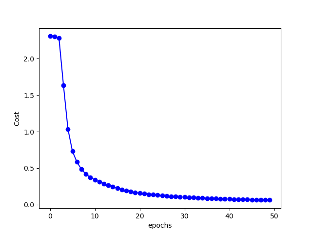
After 50 epochs of training, the accuracy on training set is: 98.41 %. Accuracy on test set is: 96.71 %. Not too shabby.
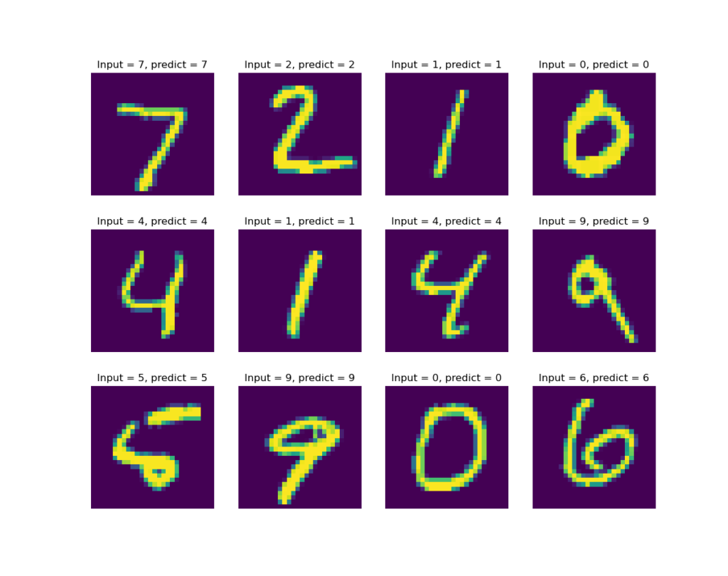
Let’s also create a few plots showing the prediction results:
nrows = 3
ncols = 4
n_plots =  nrows*ncols
fig = plt.figure(figsize=(12, 10))
for i in range(n_plots):
    axi = fig.add_subplot(nrows, ncols, i+1)
    axi.axis('off')
    xi = x_data_test[i]
    yi = y_data_test[i]
    yhati = yhat_test[i]
    plotResult(xi, yi, yhati, ax=axi)

fig.show()
It seems that at least for the first 12 test casts, our model gets them all correct. See figure below.
Lastly, the training process cost me 345 seconds, about 6 minutes. I was
using a fairly beefy 8 core AMD Ryzen 3700X desktop CPU. On a laptop
it would take a bit longer. But the performance is pretty good
considering that the entire thing uses nothing but numpy.
Wrap up
In this post, we introduced the multi-class classification neural
network. The model is trained using forward and backward
propagation. A softmax function is used as the output layer
activation, and hidden layers use logistic function as
activation. Vectorized implementation allows our simple numpy
implementation to achieve a fairly good performance.
Many of the concepts and notation are common among different types of
networks. In a future post, I will share some knowledge and
experiences in building a convolutional neural network using
numpy.
Support me
If you like the contents, please consider sending a small tip. Below this my monero wallet address:
41tR6ku6uiDA41awW1UgVD9DoJ1PxYQsMa1iQjM68ekHGTee5wgEfgLDXh7QZ3cZZnRnVuC5nGeY1Na28ZJygrHx3JeKBV7


