Table of Contents
1. What’s this about?
This is a summary with a Python implementation of an algorithm presented in this paper:
Moschopoulos, P. G., 1985: The distribution of the sum of independent gamma random variables. Annals of the Institute of Statistical Mathematics, 3, 541-544.
The problem it aims to solve is: how to fit the distribution formed by the sum of \(n\) independent Gamma random variables, with different shape and scale parameters.
Such distributions has applications in:
- queueing type problems, e.g. the total waiting time of \(X_1 + X_2 + \cdots + X_n\), where each component time \(X_i\) is distributed as Gamma.
- total excess water-flow into a dam, as \(X_1 + X_2 + \cdots + X_n\), where \(X_i\) represents the i-th excess flow at location \(i\), also distributed as Gamma.
2. Formulation of the problem
Let \(\{X_i\}, i=1, \cdots, n\) be a set of mutually independent Gamma random variables, with parameters \(\alpha_i > 0\) and \(\beta_i > 0\). The density of \(X_i\) is:
\begin{equation} \label{org43d5942} f_i (x_i; \alpha_i, \beta_i) = \frac{x_i^{\alpha_i – 1} e^{-x_i / \beta_i}}{\beta^{\alpha_i} \Gamma(\alpha_i)}, \; x_i > 0 \end{equation}where:
- \(\alpha_i > 0\): shape parameter,
- \(\beta_i > 0\): scale parameter,
- \(\Gamma()\): Gamma function.
Denote the summation of a finite number of \(n\) Gamma random variables as:
\[ Y = X_1 + X_2 + \cdots + X_n \]
We are concerned with an expression for the Probability Density Function (PDF) and Cumulative Density Function (CDF) of \(Y\), given \(\alpha_i\) and \(\beta_i\).
3. The PDF expression
I’m only giving the procedure to compute the PDF. The readers are referred to the original paper for derivation.
- Inputs:
- \(\alpha_i, i=1,2,\cdots,n\): the shape parameters of independent Gamma random variables.
- \(\beta_i, i=1,2,\cdots,n\): the scale parameters of independent Gamma random variables.
- Denote \(\beta_1 = min_i (\beta_i)\).
Compute parameter \(C\) as:
\[ C = \Pi_{i=1}^{n} (\frac{\beta_1}{\beta_i})^{\alpha_i} \]
Compute parameter \(\rho\) as:
\[ \rho = \sum_{i=1}^{n} \alpha_i \]
Compute the parameters \(\gamma_k\) as:
\[ \gamma_k = \sum_{i=1}^{n} \frac{\alpha_i (1-\beta_1/\beta_i)^k}{k} \; k=1,2,\cdots \]
Compute the weight parameters \(\delta_k\) as:
\begin{equation} \label{org9f639fc} \delta_k = \begin{cases} 1 & k = 0\\ \frac{1}{k} \sum_{i=1}^{k} i \gamma_i \delta_{k-i} & k > 0 \end{cases} \end{equation}Note that this term needs to be computed recursively.
The PDF of \(Y\) is given as a weighted sum of an infinite sequence of Gamma PDFs:
\begin{equation} \label{org57c0a7e} g(y) = C \sum_{k=0}^{\infty} \delta_k f_k(y; \rho+k, \beta_1) \end{equation}where \(f_k(y)\) is the k-th Gamma component:
\begin{equation} \label{org98d0289} f_k(y; \rho+k, \beta_1) = \frac{y^{\rho+k-1} e^{-y/\beta_1}}{\beta_1^{\rho+k} \Gamma(\rho+k)} \end{equation}
4. The CDF expression
Having got the PDF, the CDF is the term-by-term integration:
\begin{equation} \label{org9aa97fd} G(y) = C \sum_{k=0}^{\infty} \delta_k F_k(y; \rho+k, \beta_1) \end{equation}where \(F_k(y; \rho+k, \beta_1)\) is the CDF of the k-th Gamma component.
5. Truncation of the infinite sequence
In practice, both the PDF and CDF expressions take only the first \(m+1\) terms, from \(k=0\) to \(k=m\).
The paper gives the following formula for an estimation of the truncation error:
\begin{equation} \label{org00421bc} E_m(w) = \frac{C}{\beta_1^{\rho} \Gamma(\rho)} \int_{0}^{w} y^{\rho-1} e^{-y(1-b)/\beta_1} dy – G_m(w) \end{equation}where:
- \(G_m(w)\) is the sum of the first \(m+1\) terms of Equation \eqref{org9aa97fd}, for \(k=0,1,\cdots,m\).
- \(b = \max_{2 \le j \le n} (1-\beta_1/\beta_j)\).
NOTE: I wonder there is something wrong with \eqref{org00421bc}. In my experiments, the computed error bound is much too big to be meaningful. See the code and results in the next section.
I followed along the derivation but didn’t spot anything obviously wrong. My guess is that the \(b = \max_{2 \le j \le n} (1-\beta_1/\beta_j)\) upper bound is too weak, so all the subsequent inequality derivations lead to trivial constraints.
6. Python implementation
I write it into a GammaSum Class. For dependencies we need numpy
and scipy. Code below:
import numpy as np
import scipy
from scipy import stats as sstats

class GammaSum(object):
    '''Fit distribution of the sum of multiple Gamma distributions

    Args:
        alphas (ndarray or list): 1d array, shape parameters of individual
            Gamma distributions.
        betas (ndarray or list): 1d array, scale parameters of individual
            Gamma distributions. Needs to have same length as <alphas>.
        K (int): truncation level. Higher <K> value gives more accurate fits.

    Gamma distribution is defined as:
        f(x) = x^{\alpha - 1} e^{-x/\beta} / \beta^{\alpha} / \Gamma(\alpha)

    where:
        $\alpha > 0$: shape parameter,
        $\beta > 0$: scale parameter,
        $\Gamma()$: Gamma function.
    '''
    def __init__(self, alphas, betas, K):

        self.alphas = np.array(alphas).flatten()
        self.betas = np.array(betas).flatten()
        self.K = K
        self.check_params()

        # parameters to fit
        self.beta1 = None
        self.C = None
        self.rho = None
        self.gamma_k = None
        self.delta_ks = None

    def check_params(self):
        if int(self.K) != self.K:
            raise Exception("<K> needs to be a positive integer.")
        if self.K < 1:
            raise Exception("<K> should be > 1.")
        if len(self.alphas) != len(self.betas):
            raise Exception("<alphas> and <betas> need to have same size.")
        if not np.all(self.alphas > 0):
            raise Exception("<alphas> should be all > 0.")
        if not np.all(self.betas > 0):
            raise Exception("<betas> should be all > 0.")

    def compute_weights(self, K=None):
        '''Compute weights for the K Gamma distributions

        Weight for the kth Gamma:
        \delta_{k} = 1, k = 0,
        \delta_{k} = \frac{1}{k} \sum_{i=1}^{k} i \gamma_i \delta_{k-i}, k=1,2,3,...
        '''
        K = K or self.K
        # beta1
        self.beta1= np.min(self.betas)
        # C
        self.C = np.prod((self.beta1 / self.betas)**self.alphas)
        # b
        self.b = np.max((1 - self.beta1/self.betas))
        # rho
        self.rho = np.sum(self.alphas)
        # gamma_k
        self.gamma_k = self.compute_gammak()

        # weights for each gamma distr, the \delta_{k+1} term
        delta_ks = np.zeros(K+1)
        delta_ks[0] = 1.
        for k in range(K):
            if k == 0:
                delta_k1 = self.gamma_k[0]
            else:
                #delta_k1 = 0
                #for ii in range(1, k+2):
                    #delta_k1 += ii * compute_gammak(ii, self.alphas, self.betas) * delta_ks[k + 1 - ii]
                #delta_k1 /= (k+1)
                delta_k1 = np.sum(np.arange(1, k+2) * self.gamma_k[:(k+1)] * delta_ks[:(k+1)][::-1]) / (k+1)
            delta_ks[k+1] = delta_k1
        self.delta_ks = delta_ks

        return

    def compute_gammak(self, K=None):
        '''Compute the \gamma terms
        \gamma_k = \sum_{i=1}^{n} \alpha_i (1 - \beta_1/\beta_i)^k / k, k=1, 2, ...
        '''
        K = K or self.K
        kk = np.arange(1, K+2)[None, :]
        res = self.alphas[:, None] * (1 - self.beta1/self.betas[:, None])**kk / kk
        return np.sum(res, axis=0)


    def fit_pdf(self, y, K=None):
        '''Compute PDF of summed Gamma random variables

        Args:
            y (ndarray or float): values > 0.
        Keyword args:
            K (None or int): truncation level. If None, use initialized value.
        Returns:
            res (ndarary): PDF at value <y>.
        '''
        y = np.array(y)
        if not np.all(y>=0):
            raise Exception("<y> must >= 0.")

        K = K or self.K
        if self.C is None:
            self.compute_weights(K)

        res = 0
        beta1 = self.beta1
        delta_ks = self.delta_ks
        rho = self.rho
        C = self.C

        # weighted sum
        for k in range(K+1):
            dr = delta_ks[k] * y**(rho + k - 1) * np.exp(-y/beta1) / (scipy.special.gamma(rho+k) * beta1**(rho+k))
            res += dr
        res = res * C

        return res

    def fit_cdf(self, y, K=None):
        '''Compute CDF of summed Gamma random variables

        Args:
            y (ndarray or float): values > 0.
        Keyword args:
            K (None or int): truncation level. If None, use initialized value.
        Returns:
            res (ndarary): CDF at value <y>.
        '''
        y = np.array(y)
        if not np.all(y>=0):
            raise Exception("<y> must >= 0.")

        K = K or self.K
        if self.C is None:
            self.compute_weights(K)

        res = np.zeros_like(y)
        for k in range(self.K+1):
            yii = self.delta_ks[k] * sstats.gamma.cdf(y, self.rho + k, scale=self.beta1)
            res += yii
        res = res * self.C

        return res

    def estimate_error(self, y, K=None):
        '''Estimate CDF error at a given truncation level K

        NOTE: this doesn't work.
        '''
        K = K or self.K
        if self.C is None:
            self.compute_weights(K)

        y = np.array(y).flatten()
        cdf_hat = self.fit_cdf(y, K)

        def func(x, rho, b, beta1):
            return x**(rho-1) * np.exp(-x*(1-b)/beta1)

        res = np.zeros_like(y)
        for ii, yii in enumerate(y):
            intii, ee = scipy.integrate.quad(func, 0, yii, args=(self.rho, self.b, self.beta1))
            res[ii] = intii

        res = res *self.C / self.beta1**(self.rho) / scipy.special.gamma(self.rho)
        error = res - cdf_hat

        return error
7. Some sample results
Here we create 10 sets of shape and scale Gamma parameters, and for each set, randomly sample 100 points. Then we fit the summation of these 100 random samples.
Code:
# create random gamma parameters
np.random.seed(99)
alphas = np.random.rand(10) * 1
betas = np.random.rand(10) * 5
print(alphas)
print(betas)

# create random gamma rvs
N = 100
ys = []
for a, b in zip(alphas, betas):
    yii = sstats.gamma.rvs(a, scale=1/b, size=N)
    ys.append(yii)
ys = np.array(ys)

# fit gamma sum
K = 200
xx = np.linspace(0, ys.max(), 100)
gammasum = GammaSum(alphas, 1/betas, K)
gsum_pdf = gammasum.fit_pdf(xx)
gsum_cdf = gammasum.fit_cdf(xx)
error = gammasum.estimate_error(xx)

#-------------------Plot------------------------
import matplotlib.pyplot as plt
figure, ax = plt.subplots()

ax.hist(ys.sum(0), bins=20, alpha=0.6, density=True, label='hist of gamma sum')
ax.plot(xx, gsum_pdf, 'r-', label='fitted PDF')
ax.plot(xx, gsum_cdf, 'g-', label='fitted CDF')
ax.legend(loc=0)
ax.grid(True, axis='both')
ax.set_xlabel('Y')
ax.set_ylabel('PDF or CDF')

figure.show()
Note that we feed 1/betas to the GammaSum(), this is because the
paper used a different form of Gamma definition than
scipy.stats.gamma: the “scale” parameter in the paper is the
reciprocal to the “scale” parameter used in scipy.
The output figure:
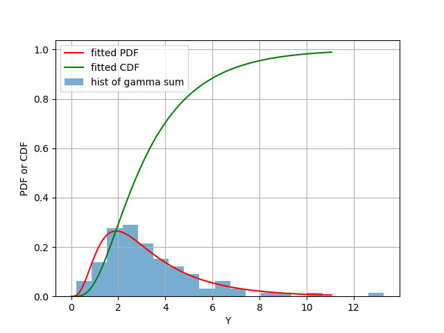

Figure 1: Blue bars: histogram of Y, as the summation of 100 random samples, sampled from 10 different Gamma random variables. Red: fitted PDF of Y. Green: fitted CDF of Y.
Note that we computed the error term but didn’t plot it. That is
because its values are way beyond reasonable range. If we plot it out
like this:
ax.hist(ys.sum(0), bins=20, alpha=0.6, density=True, label='hist of gamma sum')
ax.plot(xx, gsum_pdf, 'r-', label='fitted PDF')
ax.plot(xx, gsum_cdf, 'g-', label='fitted CDF')
ax.plot(xx, error, 'k-', label='error')
ax.legend(loc=0)
ax.grid(True, axis='both')
ax.set_xlabel('Y')
ax.set_ylabel('PDF or CDF')
This is what we got:
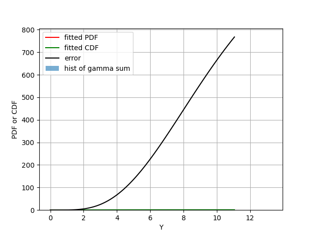

Figure 2: Similar as Fig 2 but with the additional error term as black, which dwarfs all other terms.
As I mentioned, I guess the inequality constraint is too weak, but I could be wrong. If you have a better answer, please leave a comment down below.
8. Summary
This post is short summary of a short paper:
Moschopoulos, P. G., 1985: The distribution of the sum of independent gamma random variables. Annals of the Institute of Statistical Mathematics, 3, 541-544.
The introduced algorithm is used to fit a distribution from the summation of independent Gamma random variables, with different shape and scale parameters.
Then I implemented the algorithm using numpy and scipy using Python.
Created: 2022-09-02 Fri 21:16

