
The goal
This post will share some knowledge of 2D and 3D convolutions in a
convolution neural network (CNN). Depending on the implementation,
the computational efficiency of a 2D/3D convolution can differ by a
great amount. We will be covering 3 different implementations, all
done using pure numpy and scipy, and comparing their speeds. Some
of the results will be used as building blocks for a numpy + scipy
implementation of a convolution neural network, introduced in a later
post.
Recap on convolution
If you need a recap on what 2D convolution is, here is another post where I
covered some aspects of 2D convolution, the numpy and scipy
implementations, and a Fortran implementation that deals with missing
values.
A few points that are worth reminding:
-
First and foremost, there are two similar and related operations in mathematics: convolution and cross-correlation. The difference between them is that in convolution, one flips the kernel (e.g.
kernel = kernel[::-1, ::-1]), and this flipping is not done in cross-correlation. However, in the context of machine learning and convolution neural networks, people typically use the term convolution to refer to the operation that is mathematically a cross-correlation, i.e. without the kernel flipping. Therefore, without specific notices, we will be following this convention and using the term convolution to refer the operation that does NOT involve kernel flipping. -
We will be using the term kernel and filter interchangeably.
-
In convolution neural networks, convolution is typically done in 3D, with the extra 3rd dimension being depth. More will be covered in a later post centered around CNN. For a concrete example, suppose the input image has dimensions of
(100, 100, 3), where3corresponds to the RGB channels. The kernel/filter also needs to have a depth of3, e.g.(5, 5, 3). Then the convolution is done in 3D: each time a dot product is computed between a data cube of(5, 5, 3)from the image, and the cube of the kernel itself. The kernel still strides across the image column by column and row by row, but each time a volume (rather than a slab) of data is involved in the dot product computation. -
Following the above point, we assume the image data all have a shape of
(h, w)or(h, w, c), wherehandwbeing height and width of the image, andcis the depth dimension. -
convolution can be transformed into a Fourier transform/inverse transform problem using the convolution theorem. By doing so we can leverage the powerful FFT module to speed up the computation.
-
In this context, we assume no missing data are present, so no need to worry about
nanvalues.
Padding, stride and convolution sizes
In a 2D convolution, the size of the output is \(h_o \times w_o\), where \(h_o\) is the output height, and \(w_o\) the width. All measured in number of pixels.
The output size is determined as:
\[
\left\{\begin{matrix}
h_{o} & = [(h_i + 2 p – f)/s] + 1 \\
w_{o} & = [(w_i + 2 p – f)/s] + 1 \\
\end{matrix}\right.
\]
(1)
where:
- \(h_i\) and \(w_i\) are the input sizes. For a convolution network, most of the time the images have equal heights and widths, so \(h = w\).
- \(p\) is the padding size, i.e. number of empty pixels padded onto each side of the image.
- \(f\) is the size of the convolution kernel. Again, most of the time square kernels are used, therefore the kernel width = kernel height.
- \(s\) is the stride, in both the row and column direction. A stride means the kernel makes a jump of \(s\) pixels as it travels across the columns/rows of the input image. When \(s=1\), it is a standard convolution. If \(s>1\), we are skipping some columns/rows.
- \([\,]\) is the floor function.
As a concrete example, suppose:
- input image has shape \(h_i = w_i = 28\).
- kernel size is \(f = 3\).
- padding is \(p = 0\).
- stride is \(s = 1\).
Then the output size is:
\(h_o = w_o = [(28 + 0 – 3)/1] + 1 = 26\).
Another example:
- input image has shape \(h_i = w_i = 56\).
- kernel size is \(f = 5\).
- padding is \(p = 1\).
- stride is \(s = 2\).
Then the output size is:
\(h_o = w_o = [(56 + 2 – 5)/2] + 1 = 23\).
Convolution modes
In numerical implementations, we often see that convolution has
different "modes". E.g. the numpy.convolve() function has the
following doc-string:
numpy.convolve(a, v, mode='full')
...

Parameters

    a(N,) array_like

        First one-dimensional input array.
    v(M,) array_like

        Second one-dimensional input array.

    mode{‘full’, ‘valid’, ‘same’}, optional
        ‘full’:
            By default, mode is ‘full’. This returns the convolution at each point of overlap, with an output shape of (N+M-1,). At the end-points of the convolution, the signals do not overlap completely, and boundary effects may be seen.
        ‘same’:
            Mode ‘same’ returns output of length max(M, N). Boundary effects are still visible.
        ‘valid’:
            Mode ‘valid’ returns output of length max(M, N) - min(M, N) + 1. The convolution product is only given for points where the signals overlap completely. Values outside the signal boundary have no effect.
Relating back to the size computation Equation 1 above (note that (s=1) here):
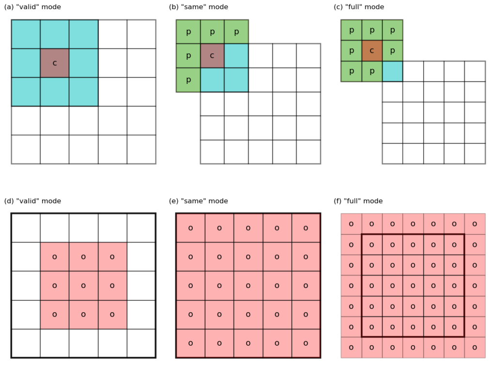
– valid mode (see Figure 1 a,d for an illustration) has \(p = 0\), and \(h_o = h_i – f + 1\). Note that the kernel never stays outside of the “valid” data domain of the input image.
– same mode (Figure 1 b,e) has \(p = (f – 1)/2\), and \(h_o = h_i + 2 p – f + 1 = h_i\), i.e. input and output have the same size. Note that some padding (labeled as p) are required to get the values around the edges of the image.
– full mode (Figure 1 c,f) does not have direct correspondence to Equation 1. However, note that the output in this mode has a size of \(h_o = h_i + f – 1\), larger than the input. The valid convolution of this output using the same kernel has a size of \(h_i + f – 1 – f + 1 = h_i\), i.e. we get back to the original size. This last observation is useful when dealing with the error back-propagation computation in a convolution neural network.
Implementing the padding function
Before moving on to the convolution implementation, let us first create a function that does the padding. See code below:
def padArray(var, pad1, pad2=None):
    '''Pad array with 0s

    Args:
        var (ndarray): 2d or 3d ndarray. Padding is done on the first 2 dimensions.
        pad1 (int): number of columns/rows to pad at left/top edges.
    Keyword Args:
        pad2 (int): number of columns/rows to pad at right/bottom edges.
            If None, same as <pad1>.
    Returns:
        var_pad (ndarray): 2d or 3d ndarray with 0s padded along the first 2
            dimensions.
    '''
    if pad2 is None:
        pad2 = pad1
    if pad1+pad2 == 0:
        return var
    var_pad = np.zeros(tuple(pad1+pad2+np.array(var.shape[:2])) + var.shape[2:])
    var_pad[pad1:-pad2, pad1:-pad2] = var

    return var_pad
Note that the function handles 2D or 3D array padding. For
instance, var1 has shape (50, 60), then padArray(var1, 1, 1)
gives an output with shape (52, 62).
If var1 has a shape of (50, 60, 3) (3 may corresponds to the RGB
channels of an image), then padArray(var1, 1, 1) gives an output
with shape (52, 62, 3).
1st conv3D() implementation: the FFT approach
Our 1st convolution implementation is based on the convolution theorem and utilizes the powerful FFT module.
The idea of this approach is:
- do the padding ourselves using the
padArray()function above. - perform a valid-mode convolution using
scipy‘sfftconvolve()function. Internally,fftconvolve()handles the convolution using FFT. - To get the correct results when stride is not 1, we only need to
pick out the result from
fftconvolve()at the same stride.
See code below:
def checkShape(var, kernel):
    '''Check shapes for convolution

    Args:
        var (ndarray): 2d or 3d input array for convolution.
        kernel (ndarray): 2d or 3d convolution kernel.
    Returns:
        kernel (ndarray): 2d kernel reshape into 3d if needed.
    '''
    var_ndim = np.ndim(var)
    kernel_ndim = np.ndim(kernel)

    if var_ndim not in [2, 3]:
        raise Exception("<var> dimension should be in 2 or 3.")
    if kernel_ndim not in [2, 3]:
        raise Exception("<kernel> dimension should be in 2 or 3.")
    if var_ndim < kernel_ndim:
        raise Exception("<kernel> dimension > <var>.")
    if var_ndim == 3 and kernel_ndim == 2:
        kernel = np.repeat(kernel[:, :, None], var.shape[2], axis=2)

    return kernel

def pickStrided(var, stride):
    '''Pick sub-array by stride

    Args:
        var (ndarray): 2d or 3d ndarray.
        stride (int): stride/step along the 1st 2 dimensions to pick
            elements from <var>.
    Returns:
        result (ndarray): 2d or 3d ndarray picked at <stride> from <var>.
    '''
    if stride < 0:
        raise Exception("<stride> should be >=1.")
    if stride == 1:
        result = var
    else:
        result = var[::stride, ::stride, ...]
    return result

  def conv3D(var, kernel, stride=1, pad=0):
      '''3D convolution using scipy.signal.fftconvolve.

      Args:
          var (ndarray): 2d or 3d array to convolve along the first 2 dimensions.
          kernel (ndarray): 2d or 3d kernel to convolve. If <var> is 3d and <kernel>
              is 2d, create a dummy dimension to be the 3rd dimension in kernel.
      Keyword Args:
          stride (int): stride along the 1st 2 dimensions. Default to 1.
          pad (int): number of columns/rows to pad at edges.
      Returns:
          conv (ndarray): convolution result.
      '''
      stride = int(stride)
      kernel = checkShape(var, kernel)
      if pad > 0:
          var_pad = padArray(var, pad, pad)
      else:
          var_pad = var

      conv = fftconvolve(var_pad, kernel, mode='valid')
      if stride > 1:
          conv = pickStrided(conv, stride)

      return conv
Here, checkShape() is doing some input sanity checks,
and pickStrided() picks out the desired output at given strides.
2nd conv3D() implementation: the sub-matrix approach
This approach is inspired by a Stackoverflow answer. The name
"sub-matrix" is informal (the author of the above SO answer called it
specialconvolve), and is chosen here due to its sub-matrix slicing
operations.
As a concrete example, suppose the input matrix is (10, 10), and the
convolution kernel is (3, 3). It is easy to work out that the output
will have a shape of (8, 8).
See the Figure below for an illustration of the process.
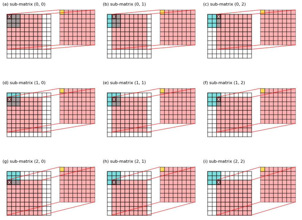
To get this output, we make 3 * 3 = 9
sub-matrix slices from the original input, each has a size of (8, 8), and multiple that slab with one value from the kernel.
More formally:
- set
i = 0andj = 0, the value from the kernel at index(i, j)is denotedkernel[i, j](labeledxin Figure 2a). - take a slice from the input image as
image[i : i+8, j : j+8], and multiple it withkernel[i, j]to giveslabij = image[i : i+8, j : j+8] * kernel[i, j](red slab on the right in Figure 2a). - add this
slabijto an accumulator variable:result = result + slabij. - increment
jby 1 and repeat steps 2-3, do this tillj == 2. (First row in Figure 2). - increment
iby 1 and repeat steps 2-3-4, do this tilli == 2.
Notice that during this process, the 9 cells in the top left corner
are contributing to the final convolution output, labeled yellow on
the right slab.
Th number of dot product
computations is 3 * 3 = 9, instead of 8 * 8 = 64. Each time, a
bigger (8, 8) slab is involved in the dot product, rather than a
smaller one as big as the kernel ((3, 3)). This better utilizes the
vectorized matrix operation of numpy and saves a considerable amount
of time. The author of the SO answer claimed a 1000 times speed up
compared with scipy.signal.convolve2d(), and I also noticed that it
works particularly well when the kernel size is very small. More on
speed comparisons will be given in a later section.
The code is given below:
def conv3D2(var, kernel, stride=1, pad=0):
    '''3D convolution by sub-matrix summing.

    Args:
        var (ndarray): 2d or 3d array to convolve along the first 2 dimensions.
        kernel (ndarray): 2d or 3d kernel to convolve. If <var> is 3d and <kernel>
            is 2d, create a dummy dimension to be the 3rd dimension in kernel.
    Keyword Args:
        stride (int): stride along the 1st 2 dimensions. Default to 1.
        pad (int): number of columns/rows to pad at edges.
    Returns:
        result (ndarray): convolution result.
    '''
    var_ndim = np.ndim(var)
    ny, nx = var.shape[:2]
    ky, kx = kernel.shape[:2]
    result = 0
    if pad > 0:
        var_pad = padArray(var, pad, pad)
    else:
        var_pad = var

    for ii in range(ky*kx):
        yi, xi = divmod(ii, kx)
        slabii = var_pad[yi:2*pad+ny-ky+yi+1:1,
                         xi:2*pad+nx-kx+xi+1:1, ...]*kernel[yi, xi]
        if var_ndim == 3:
            slabii = slabii.sum(axis=-1)
        result += slabii

    if stride > 1:
        result = pickStrided(result, stride)

    return result
Notice that again, we do the padding ourselves using the padArray()
function, and pick out the strided values using pickStrided(). Also,
it works for either 2D or 3D data.
3rd conv3D() implementation: the stride-view approach
The 3rd approach uses a fairly hidden function in numpy —
numpy.lib.stride_tricks.as_strided() — to achieve a vectorized
computation of all the dot product operations in a 2D or 3D
convolution.
Recall that in a 2D convolution, we slide the kernel across the input image, and at each location, compute a dot product and save the output.
For instance, the input image has a shape of (10, 10), and the
kernel is (3, 3). Then at each row, there is 10 - 3 + 1 = 8
locations where the kernel overlaps with the image, giving 8 dot
product computations. After iterating through all rows, the output has
a shape of (8, 8).
Now imagine for each of these 8 * 8 = 64 locations, we obtain a 3 * 3
slab from the input image, and stack them all up in a big
pile and name it view. See Figure 3 below for an illustration of
the first 6 slabs in the pile.
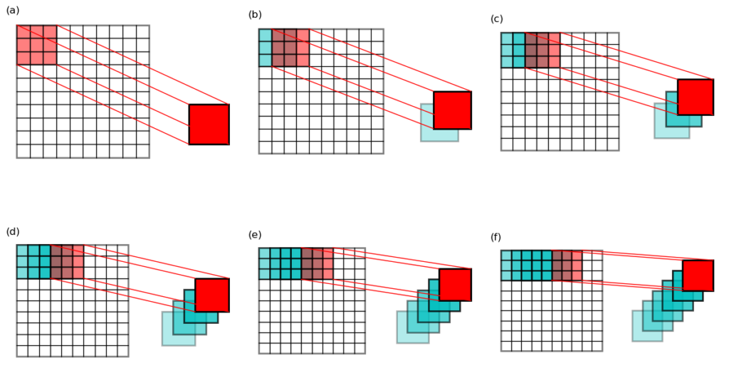
This pile will have a shape of (64, 3, 3). You may already know that
in numpy, when multiplying one variable of shape (64, 3, 3)
and one with shape (3, 3), a broadcasting of the latter variable
automatically happens such that it is like multiplying (element-wise)
two (64, 3, 3) variables together.
To express this process using some Python code, suppose:
viewis anndarraywith shape(64, 3, 3).kernelis anndarraywith shape(3, 3).
Then the result of
prod = view * kernel
is the same as these:
kernel_broadcasted = np.repeat(kernel[None, :, :], 64, axis=0)  # kernel_broadcasted is (64, 3, 3)
prod = view * kernel_broadcasted
Then it is easy to get the convolution result by summing up the last 2 dimensions:
conv = np.sum(prod, axis=(1, 2)) # conv shape is (64,)
Lastly, we only need to reshape this conv into a shape of (8, 8):
conv = conv.reshape((8, 8))
It is noticed that the core of this trick lies in the construction of
the that big "pile" of matrix slices, and this is achieved using the
above mentioned numpy.lib.stride_tricks.as_strided() function.
I will leave it to the reader to figure out how this trick works.
Below is the code of this 3rd convolution implementation:
def asStride(arr, sub_shape, stride):
    '''Get a strided sub-matrices view of an ndarray.

    Args:
        arr (ndarray): input array of rank 2 or 3, with shape (m1, n1) or (m1, n1, c).
        sub_shape (tuple): window size: (m2, n2).
        stride (int): stride of windows in both y- and x- dimensions.
    Returns:
        subs (view): strided window view.

    See also skimage.util.shape.view_as_windows()
    '''
    s0, s1 = arr.strides[:2]
    m1, n1 = arr.shape[:2]
    m2, n2 = sub_shape[:2]

    view_shape = (1+(m1-m2)//stride, 1+(n1-n2)//stride, m2, n2)+arr.shape[2:]
    strides = (stride*s0, stride*s1, s0, s1)+arr.strides[2:]
    subs = np.lib.stride_tricks.as_strided(
        arr, view_shape, strides=strides, writeable=False)

    return subs

def conv3D3(var, kernel, stride=1, pad=0):
    '''3D convolution by strided view.

    Args:
        var (ndarray): 2d or 3d array to convolve along the first 2 dimensions.
        kernel (ndarray): 2d or 3d kernel to convolve. If <var> is 3d and <kernel>
            is 2d, create a dummy dimension to be the 3rd dimension in kernel.
    Keyword Args:
        stride (int): stride along the 1st 2 dimensions. Default to 1.
        pad (int): number of columns/rows to pad at edges.
    Returns:
        conv (ndarray): convolution result.
    '''
    kernel = checkShape(var, kernel)
    if pad > 0:
        var_pad = padArray(var, pad, pad)
    else:
        var_pad = var

    view = asStride(var_pad, kernel.shape, stride)
    if np.ndim(kernel) == 2:
        conv = np.sum(view*kernel, axis=(2, 3))
    else:
        conv = np.sum(view*kernel, axis=(2, 3, 4))

    return conv
Here, the asStride() function is responsible for creating that big
"pile". Using the above example, the return value of subs will have
a shape of (8, 8, 3, 3).
Then in the conv3D3() function, the dot products in the convolution
is computed in
conv = np.sum(view*kernel, axis=(2, 3))
giving a result conv with shape (8, 8).
Notice that when using the strided-view trick, the last
reshaping from (64,) to (8, 8) array is not even necessary,
because we can construct the view directly into a shape of (8, 8, 3, 3), and the dot product operation happens at the last 2
dimensions.
Also note that it also works when the stride is not 1, and when the input and kernel are 3D.
When the stride is smaller than the kernel size (which is typically the case), it is easy to notice that there are many duplicated values in the "pile". Or even more precisely, there are many mirrored locations in the strided-view, and each group of mirrored locations share the same value in memory. The number of locations in the pile will be the same as the input image only when the stride equals the kernel size (i.e. non-overlapping convolution).
Lastly, this strided-view trick can also be used during the pooling process. More on pooling will be covered in a separate post.
One additional word of warning: according to the numpy
documentation, it is regarded as dangerous to write into the
as_strided() output:
Furthermore, arrays created with this function often contain self
overlapping memory, so that two elements are identical. Vectorized
write operations on such arrays will typically be unpredictable. They
may even give different results for small, large, or transposed
arrays. Since writing to these arrays has to be tested and done with
great care, you may want to use `writeable=False` to avoid accidental
write operations.

For these reasons it is advisable to avoid `as_strided` when possible.
Comparing different implementations
We have introduced 3 different implementations of 2D or 3D convolution using
numpy or scipy:
conv3D(), usingscipy.signal.fftconvolve().conv3D2(), using sub-matrix slices.conv3D3(), using strided-view of anndarray.
I did some comparisons on the speeds of these 3 methods, using inputs and kernels of different sizes. The results are given in this SO answer. Here is an image showing the speed comparison results.
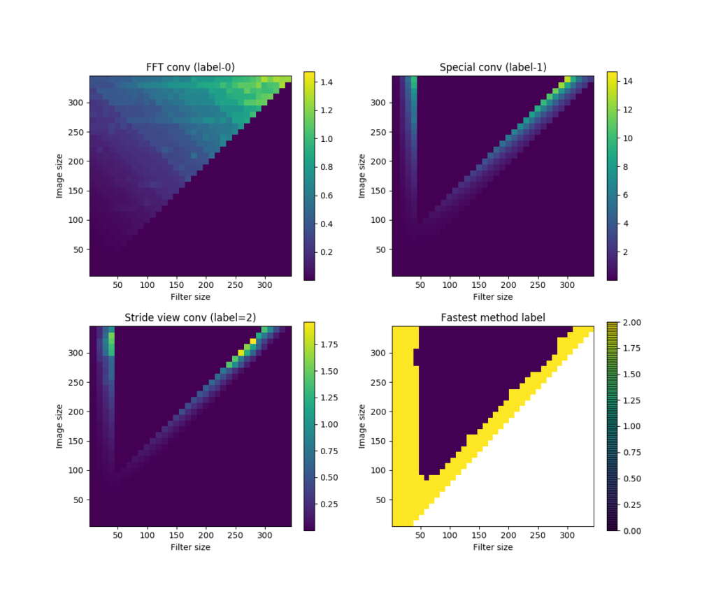
nxnx5, kernel shape=fxfx5. Computations in each method are repeated for 10 times. (a) shows the time took by the FFT convolution method (labeled 0), (b) the sub-matrix method (labeled 1), and (c) the strided-view method (labeled 2). (d) shows the label of the winner method in each input-kernel size combination.To summarize:
conv3D()is in general the fastest.conv3D2()andconv3D3()get slow as kernel size increases, but faster again as the kernel size approaches the size of input data.conv3D2()has advantages for very small kernels (smaller than about 5 x 5).conv3D3()is the fastest when kernel size approaches input.
If you like the contents, please consider sending a small tip. Below this my monero wallet address:
41tR6ku6uiDA41awW1UgVD9DoJ1PxYQsMa1iQjM68ekHGTee5wgEfgLDXh7QZ3cZZnRnVuC5nGeY1Na28ZJygrHx3JeKBV7


