Rationale
2D convolution can be used to perform moving average/smoothing,
gradient computation/edge detection or the computation of Laplacian
(which is the 2nd order derivative) etc.. This can be
achieved using the scipy.signal.convolve2d, scipy.signal.convolve,
scipy.signal.fftconvolve or
scipy.ndimage.convolve functions in Python. However, there is a catch in all
these methods: If your data contain any missing value (e.g. nan),
the convolved result will have an enlarged hole around each missing
data point. That is to say, any overlap between the missing value and
the kernel being convolved will create a missing in the output. An
example is given below.
scipy.ndimage.convolve(). (c) similar as (b) but using scipy.signal.convolve2d(). (d) similar as (b) but using scipy.signal.fftconvolve(). (e) similar as (b) but using scipy.signal.convolve(). (f) similar as (b) but using a custom convolve2D() function. (g) similar as (b) but using a custom convolve2DFFT() function.Figure 1a displays a random field generated from a standard Gaussian:
data = np.random.randn(30, 30)
Along the diagonal line, there are 3 blocks of missing values
(np.nan) with sizes of 1x1, 3x3 and 5x5:
data[5, 5] = np.nan
data[12:15, 12:15] = np.nan
data[20:25, 20:25] = np.nan
These are represented by white color in Figure 1a.
Figure 1b shows the result of 2d
convolution with a 5x5 kernel (with all 1s in the 5x5 array)
using the scipy.ndimage.convolve() function:
r1=scipy.ndimage.convolve(data, kernel, mode='constant',cval=0.)
It can be seen that the missing holes in the original data get
inflated in the convolution result, because of the overlaps between
nan values and the kernel.
In some cases this might be the desired result: it is required that
100 % of the data in each convolution step need to be present and
valid to compute a legitimate result. In the case of a moving average,
this is requiring that all data points are present and valid in a
local neighborhood to compute the neighborhood mean.
However, in other cases this might be too strict a requirement. Maybe some
degrees of data loss is tolerable, for instance, you require only at
least 50% of the neighborhood data to compute a neighborhood
average. For such kind of forgiving tolerance, the scipy.ndimage.convolve()
function would result in a big loss of data, and doesn’t utilize
the existing information contained in the data very well.
Figure 1 also shows the results using other convolution functions in
scipy.
Figure 1c – 1e are computed using these functions:
r2 = scipy.signal.convolve2d(data, kernel, mode='same')
r3 = scipy.signal.fftconvolve(data, kernel, mode='same')
r4 = scipy.signal.convolve(data, kernel, mode='same')
scipy.signal.convolve2d (Figure 1c) gives the same
result as scipy.ndimage.convolve (Figure
1b). scipy.signal.fftconvolve produces a slab of nans, because the
convolution is done in the frequency space using the convolution theorem. By default, scipy.signal.convolve calls a
choose_conv_method() to determine how to compute the
convolution. Apparently in this case it chose the FFT approach and
resulted in a slab of nans (Figure 1d).
None of these scipy functions give ideal solutions. Therefore our goal is
to look for some alternative convolution methods that allow
some controllable level of tolerance to missing data.
Algorithm design
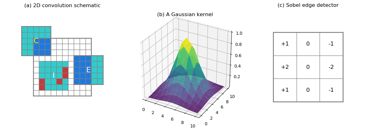
As we slide the convolution kernel across the data, at each location
(i, j) of the data domain the kernel defines a neighborhood within which the
corresponding values in the kernel and the data are multiplied and the
products summed. At the edge or corner of the data domain (Figure 2a,
Label E and C, respectively), there are
fewer overlapping values than in the interior. When computing the
proportion of missing values in the neighborhood, we would like to
take this edge-interior difference into account. For instance, the
corner case (C) in Figure 2a covers only 9 valid data points (at
most, without any missing), and
the edge case (E) covers at most 15 data points out of 25.
In the interior case (I), 5 missing values are represented by red
squares, and they constitute 20% of the kernel size. Whether this
proportion of missing is tolerable for the computation at location
I is subject to the user. We need to provide the user with
a max_missing input argument to control this behavior: if the
proportion of missing values within an overlap neighborhood exceeds
max_missing, the convolution result is set to nan, signaling "not having
enough information here".
The kernel can contain arbitrary values. For instance, a Gaussian kernel
puts higher weights at the kernel center (see Figure 2b). Or, a Sobel
edge detection kernel like shown in Figure 2c (only the horizontal
component). 0s in the kernel indicate no contribution from these points,
therefore, if a 0 in the kernel overlaps with a nan in the data
domain, it should not cause any damage to the computation, since we
are not counting the 0s anyways. On the other hand, one may want to be
more specific about what are counted as 0s in the kernel. Like the
Gaussian surface shown in Figure 2b, its value drops towards 0 fairly
quickly around the edges, should a, say, 0.00004 be rounded to 0?
To clarify such ambiguity, we require one more binary input argument
that informs the algorithm about the locations of valid kernel values with 1s,
and empty locations with 0s.
A Fortran solution
Big, nested loops in Python should be avoided as much as possible, as the speed would be quite pathetic. In case of absolute necessity, one should try an implementation using C or Fortran and compile an extension module for Python, or implement the algorithm in Cython. Here I show a Fortran solution:
module CONV2D
implicit none

private
public CONVOLVE2D, RUNMEAN2D
contains

    !--------Convolve 2d slab with given kernel--------
    subroutine CONVOLVE2D(slab,slabmask,kernel,kernelflag,max_missing,resslab,resmask,hs,ws)
        ! Convolve 2d slab with given kernel

        ! <slab>: real, 2d input array.
        ! <slabmask>: int, 2d mask for <slab>, 0 means valid, 1 means missing/invalid/nan.
        ! <kernel>: real, 2d input array with smaller size than <slab>, kernel to convolve with.
        ! <kernelflag>: int, 2d flag for <kernel>, 0 means empty, 1 means something. This is
        !               to fercilitate counting valid points within element.
        ! <max_missing>: real, max percentage of missing within any convolution element tolerable.
        !                E.g. if <max_missing> is 0.5, if over 50% of values within a given element
        !                are missing, the center will be set as missing (<res>=0, <resmask>=1). If
        !                only 40% is missing, center value will be computed using the remaining 60%
        !                data in the element.
        ! <hs>, <ws>: int, height and width of <slab>. Optional.
        !
        ! Return <resslab>: real, 2d array, result of convolution.
        !        <resmask>: int, 2d array, mask of the result. 0 means valid, 1 means missing (no
        !                   enough data within element).

        implicit none
        integer, parameter :: ikind = selected_real_kind(p=15,r=10)

        integer :: hs, ws
        real(kind=ikind), dimension(hs,ws), intent(in) :: slab
        real(kind=ikind), dimension(hs,ws), intent(out) :: resslab
        integer, dimension(hs,ws), intent(in) :: slabmask
        integer, dimension(hs,ws), intent(out) :: resmask
        real(kind=ikind), dimension(:,:), intent(inout) :: kernel
        integer, dimension(:,:), intent(inout) :: kernelflag
        real, intent(in) :: max_missing

        integer :: hk, wk, ii, jj, i, j, nvalid, nbox
        integer :: hw_l, hw_r, hh_u, hh_d, x1, x2, y1, y2
        real(kind=ikind) :: tmp

        !--------Default values--------
        resslab=0.
        resmask=1

        !-------------------Check shape-------------------
        hk=size(kernel,1)    ! height of kernel
        wk=size(kernel,2)    ! width of kernel

        if (hk /= size(kernelflag,1) .OR. wk /= size(kernelflag,2)) then
            write(*,*) 'Shape do not match between <kernel> and <kernelflag>.'
            return
        end if

        if ( hk >= hs .OR. wk >= ws) then
            write(*,*) 'kernel too large.'
            return
        end if

        if (max_missing <=0 .OR. max_missing >1) then
            write(*,*) '<max_missing> needs to be in range (0,1].'
            return
        end if

        !-------------------Flip kernel-------------------
        kernel=kernel(ubound(kernel,1):lbound(kernel,1):-1, ubound(kernel,2):lbound(kernel,2):-1)
        kernelflag=kernelflag(ubound(kernelflag,1):lbound(kernelflag,1):-1, &
            & ubound(kernelflag,2):lbound(kernelflag,2):-1)

        !---------------Half kernel lengths---------------
        if (mod(hk,2) == 1) then
            hh_u=(hk-1)/2
            hh_d=(hk-1)/2
        else
            hh_u=hk/2-1
            hh_d=hk/2
        end if

        if (mod(wk,2) == 1) then
            hw_l=(wk-1)/2
            hw_r=(wk-1)/2
        else
            hw_l=wk/2-1
            hw_r=wk/2
        end if

        !-------------------Loop through grids-------------------
        do ii = 1,hs
            do jj = 1,ws
                y1=ii-hh_u
                y2=ii+hh_d
                x1=jj-hw_l
                x2=jj+hw_r
                tmp=0.
                nvalid=0
                nbox=0

                do i = y1,y2
                    do j = x1,x2
                        ! skip out-of-bound points
                        if (i<1 .or. i>hs .or. j<1 .or. j>ws) then
                            cycle
                        end if
                        nvalid=nvalid+(1-slabmask(i,j))*kernelflag(i-y1+1,j-x1+1)
                        tmp=tmp+(1-slabmask(i,j))*slab(i,j)*kernel(i-y1+1,j-x1+1)
                        nbox=nbox+kernelflag(i-y1+1,j-x1+1)
                    end do
                end do

                if (1-float(nvalid)/nbox < max_missing) then
                    resslab(ii,jj)=tmp
                    resmask(ii,jj)=0
                else
                    resslab(ii,jj)=0.
                    resmask(ii,jj)=1
                end if
            end do
        end do
    end subroutine CONVOLVE2D
The code is put in a Fortran module CONV2D, which contains 2 public
subroutines: CONVOLVE2D and RUNMEAN2D. I’m only showing the
former, the latter can be easily created based on CONVOLVE2D.
There are 5 arguments to the CONVOLVE2D subroutine that are
intent(in):
slab: the 2d data array.slabmask: a binary array with1s indicting missing values inslab.kernel: convolution kernel.kernelflag: a binary array with0s indicting empty locations inkernel,1s otherwise.max_missing: a float in(0, 1), the maximum tolerable proportion of missing values in each neighborhood.
The subroutine has 2 intent(out) arguments:
resslab: the convoluted 2d array.resmask: a binary array with1s indicting missings inresslab.
Nothing too complicated inside the subroutine, we are doing a standard
convolution process. The only difference is that the number of missing
values in each neighborhood is counted (nvalid), and the proportion
of missings to the maximum possible valid numbers (nbox) are
computed, and the result compared with the given threshold:
if (1-float(nvalid)/nbox < max_missing) then
    resslab(ii,jj)=tmp
    resmask(ii,jj)=0
else
    resslab(ii,jj)=0.
    resmask(ii,jj)=1
Also don’t forget to flip the kernel, otherwise it would be a cross-correlation rather than convolution:
kernel=kernel(ubound(kernel,1):lbound(kernel,1):-1, ubound(kernel,2):lbound(kernel,2):-1)
kernelflag=kernelflag(ubound(kernelflag,1):lbound(kernelflag,1):-1, &
    & ubound(kernelflag,2):lbound(kernelflag,2):-1)
Lastly, one can use f2py to compile the Fortran code into a Python module. For more information regarding this process, check out this post Use f2py to compile Python module.
The result of
r5 = convolve2D(data, kernel, max_missing=0.9)
is shown in Figure 1f. We are allowing up to 90%
missing in each neighborhood, therefore the smaller holes of missing
values are filled up completely, and the larger 5x5 missing hole
shrinks to a single pixel. Because a 5x5 convolution kernel cannot provide
> 10 % valid data to a 5x5 missing box, there is 1 missing left at
the center. You can make a 2D moving average function out from this,
and use it to fill-up some missings values with available neighborhood averages.
An FFT solution
Convolution can be achieved by multiplying the Fourier transforms of the two convolving signals, then applying the inverse Fourier transform on the product:
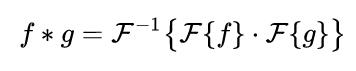
Computation of Fourier transforms can be further boosted by the
FFT algorithm. Therefore, convolution using the FFT approach is
typically faster, depending on the sizes of the convolving signals. My
experience is that when the kernel (say, g) is not too small (bigger than
2x2, or 3x3), nor too large (not nearly as large as f), the FFT
approach is faster than the Fortran solution shown above.
Here is the Python implementation using scipy:
def convolve2DFFT(slab,kernel,max_missing=0.5,verbose=True):
    '''2D convolution using fft.

    <slab>: 2d array, with optional mask.
    <kernel>: 2d array, convolution kernel.
    <max_missing>: real, max tolerable percentage of missings within any
                   convolution window.
                   E.g. if <max_missing> is 0.5, when over 50% of values
                   within a given element are missing, the center will be
                   set as missing (<res>=0, <resmask>=1). If only 40% is
                   missing, center value will be computed using the remaining
                   60% data in the element.
                   NOTE that out-of-bound grids are counted as missings, this
                   is different from convolve2D(), where the number of valid
                   values at edges drops as the kernel approaches the edge.

    Return <result>: 2d convolution.
    '''
    from scipy import signal

    assert np.ndim(slab)==2, "<slab> needs to be 2D."
    assert np.ndim(kernel)==2, "<kernel> needs to be 2D."
    assert kernel.shape[0]<=slab.shape[0], "<kernel> size needs to <= <slab> size."
    assert kernel.shape[1]<=slab.shape[1], "<kernel> size needs to <= <slab> size."

    #--------------Get mask for missings--------------
    slabcount=1-np.isnan(slab)

    # this is to set np.nan to a float, this won't affect the result as
    # masked values are not used in convolution. Otherwise, nans will
    # affect convolution in the same way as scipy.signal.convolve()
    # and the result will contain nans.
    slab=np.where(slabcount==1,slab,0)
    kernelcount=np.where(kernel==0,0,1)

    result=signal.fftconvolve(slab,kernel,mode='same')
    result_mask=signal.fftconvolve(slabcount,kernelcount,mode='same')

    valid_threshold=(1.-max_missing)*np.sum(kernelcount)
    result=np.where(result_mask<valid_threshold,result,np.nan)
    #NOTE: the number of valid point counting is different from convolve2D(),
    #where the total number of valid points drops as the kernel moves to the
    #edges. This can be replicated here by:
    # totalcount=signal.fftconvolve(np.ones(slabcount.shape),kernelcount,
    # mode='same')
    # valid_threshold=(1.-max_missing)*totalcount
    #But will involve doing 1 more convolution.
    #Another way is to convolve a small matrix (big enough to get the drop
    #at the edges, and set the same numbers to the totalcount.

    return result
Basically 2 separate convolutions are performed:
- convolution of the data and the kernel:
result = signal.fftconvolve(slab, kernel, mode='same')
- convolution of the binary valid data flag and the binary valid
kernel flag (for both,
0for missing,1otherwise):
result_mask = signal.fftconvolve(slabcount, kernelcount, mode='same')
Then those grid boxes where the valid data number in its neighborhood
is smaller than the missing level specified by max_missing are replaced
by nan:
valid_threshold = (1.-max_missing)*np.sum(kernelcount)
result = np.where(result_mask<valid_threshold, result, np.nan)
The result of calling
r6 = convolve2DFFT(data, kernel, max_missing=0.9)
is shown in Figure 1g. Again, the 2 smaller missing holes are filled up completely, and the larger hole lefts 1 missing.


