Intro
Some time ago I saw a gif animation online showing someone doing a replica of the Mona Lisa in a "spiral" way. He/she keeps on drawing a continuous, tightly packed-up spiral curve from the center of the canvas outwards, using a calligraphy brush to create varying thickness of the line stroke. In the end you see the image of Mona Lisa, it is like a Mosaic art but in the polar coordinate. I thought I could probably do the similar thing, but with the power of a programming language. So here is an attempt in Python.
The Python script
Post the script first:
FILE_IN='people01.jpg'
dr1=4.5
dr2=4
lseg=4
nlayers=4
sigma=3

import numpy as np
from PIL import Image
from PIL import ImageFilter
import matplotlib.pyplot as plt

if __name__=='__main__':

    #-----------Read in image----------------------
    img=Image.open(FILE_IN).convert('L')

    # resize
    newsize=(300, int(float(img.size[1])/img.size[0]*300))
    img=img.resize(newsize,Image.ANTIALIAS)
    print('Image size: %s' %str(img.size))

    # blur
    img=img.filter(ImageFilter.GaussianBlur(sigma))

    # convert to array
    img=np.array(img)
    img=img[::-1,:]

    # thresholding
    layers=np.linspace(np.min(img),np.max(img),nlayers+1)
    img_layers=np.zeros(img.shape)
    ii=1
    for z1,z2 in zip(layers[:-1],layers[1:]):
        img_layers=np.where((img>=z1) & (img<z2),ii,img_layers)
        ii+=1
    img_layers=img_layers.max()-img_layers+1

    # get diagonal length
    size=img.shape # ny,nx
    diag=np.sqrt(size[0]**2/4+size[1]**2/4)

    figure=plt.figure(figsize=(12,10),dpi=100)
    ax=figure.add_subplot(111)

    # create spiral
    rii=1.0
    line=np.zeros(img.shape)
    nc=0
    while True:
        if nc==0:
            rii2=rii+dr1
        else:
            rii=rii2
            rii2=rii+dr2

        print('r = %.1f' %rii)
        nii=max(64,2*np.pi*rii//lseg)
        tii=np.linspace(0,2*np.pi,nii)
        riis=np.linspace(rii,rii2,nii)
        xii=riis*np.cos(tii)
        yii=riis*np.sin(tii)

        if np.all(riis>=diag):
            break

        # get indices
        xidx=np.around(xii,0).astype('int')+size[1]//2
        yidx=np.around(yii,0).astype('int')+size[0]//2
        idx=[jj for jj in range(len(yidx)) if xidx[jj]>=0 and yidx[jj]>=0\
                and xidx[jj]<=size[1]-1 and yidx[jj]<=size[0]-1]
        xidx=xidx[idx]
        yidx=yidx[idx]

        # skip diagonal jumps
        if len(yidx)>0 and yidx[0]*yidx[-1]<0:
            continue
        xii=xii[idx]
        yii=yii[idx]

        # pick line width from image
        lw=img_layers[yidx,xidx]

        # add random perturbation
        lwran=np.random.random(lw.shape)-0.5
        lw=lw+lwran

        # randomize color
        colorjj=np.random.randint(0,60)*np.ones(3)/float(255)

        for jj in range(len(xii)-1):

            # smooth line widths
            lwjjs=lw[max(0,jj-3):min(len(lw),jj+3)]
            if jj==0 and nc>0:
                lwjjs=np.r_[lwjjs_old,lwjjs]

            wjj=np.ones(len(lwjjs))
            wjj=wjj/len(wjj)
            lwjj=np.dot(lwjjs,wjj)

            ax.plot([xii[jj], xii[jj+1]],
                    [yii[jj], yii[jj+1]],
                    color=colorjj,
                    linewidth=lwjj)

            if jj==len(xii)-2:
                lwjjs_old=lwjjs

        nc+=1

    ax.axis('off')
    ax.set_facecolor((1.,0.5,0.5))
    ax.set_aspect('equal')
    figure.show()
Break down of the script
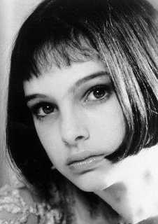
To create a "spiral replica" of some image/painting we first need to
load a digital copy of the reference image.
(The image file used in the script can be
obtained from here.)
I used the PIL package
for this, and re-scaled it to a predefined width of 300
to reduce the amount of details and the computational cost:
from PIL import Image
img = Image.open(FILE_IN).convert('L')
newsize = (300, int(float(img.size[1])/img.size[0]*300))
img = img.resize(newsize, Image.ANTIALIAS)
The .convert('L') function converts the color image to greyscale,
using this formula:
L = R * 299/1000 + G * 587/1000 + B * 114/1000
Then I did a Gaussian blur on the greyscale image, again to reduce the high frequency details:
img = img.filter(ImageFilter.GaussianBlur(sigma))
The sigma parameter is defined at the top of the script, you can
adjust it yourself.
After converting the image to numpy array, I segmented the greyscale
intensities of the image into a number of layers:
layers=np.linspace(np.min(img), np.max(img), nlayers+1)
Such layers will be used to control the width of the spiral curve: the lower the greyscale intensity (lower intensity corresponds to darker color), the thicker the line stroke:
img_layers=np.zeros(img.shape)
ii=1
for z1,z2 in zip(layers[:-1],layers[1:]):
	img_layers=np.where((img>=z1) & (img<z2),ii,img_layers)
	ii+=1
img_layers=img_layers.max()-img_layers+1
The spirals are created in the big while True loop, the number of
circles is recorded in the nc variable.
In each cycle we define the starting radius (using the center of the
image as origin) as rii and the finishing radius after a 360 degree
rotation as rii2. rii2 > rii so it spirals outwards.
In the 1st cycle (nc=0), the starting and finish radii are rii
and rii+dr1, respectively. For subsequent circles the increase of
radius in each cycle is dr2. I defined dr1 and dr2 separately
because the first cycle of the spiral tends to create a big solid dot
at the center of the image so a slightly bigger dr1 can help remove
the big solid dot.
During each cycle the spiral curve is broken down into a number line
segments, each with a length of lseg; or the number of segments is
set to 64, whichever way gives a larger segment number. Then the 2 pi cycle is segmented accordingly, and the x, y coordinates obtained from the linearly interpolated radius riis:
nii = max(64, 2*np.pi*rii//lseg)
tii = np.linspace(0, 2*np.pi, nii)
riis = np.linspace(rii, rii2, nii)
xii = riis*np.cos(tii)
yii = riis*np.sin(tii)
Then I rounded the xii, yii coordinates to the nearest integers,
which are used as indices to index the line width values at the
underlying pixels:
xidx=np.around(xii,0).astype('int')+size[1]//2
yidx=np.around(yii,0).astype('int')+size[0]//2
idx=[jj for jj in range(len(yidx)) if xidx[jj]>=0 and yidx[jj]>=0\
	and xidx[jj]<=size[1]-1 and yidx[jj]<=size[0]-1]
xidx=xidx[idx]
yidx=yidx[idx]

# skip diagonal jumps
if len(yidx)>0 and yidx[0]*yidx[-1]<0:
	continue
xii=xii[idx]
yii=yii[idx]

# pick line width from image
lw=img_layers[yidx,xidx]
A random perturbation is given to the sampled line widths, and the line colors, to give a more natural looking curve:
lwran=np.random.random(lw.shape)-0.5
lw=lw+lwran
colorjj=np.random.randint(0,60)*np.ones(3)/float(255)
However, this still creates jagged line segments. Therefore I further smoothed the line widths with a 3-unit moving average:
for jj in range(len(xii)-1):

	# smooth line widths
	lwjjs=lw[max(0,jj-3):min(len(lw),jj+3)]
	if jj==0 and nc>0:
	lwjjs=np.r_[lwjjs_old,lwjjs]

	wjj=np.ones(len(lwjjs))
	wjj=wjj/len(wjj)
	lwjj=np.dot(lwjjs,wjj)
Lastly, the line segments are plotted using matplotlib.
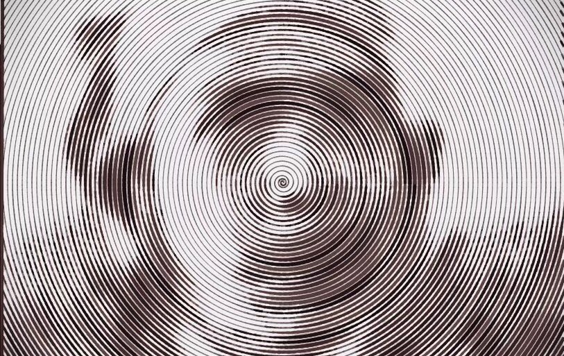
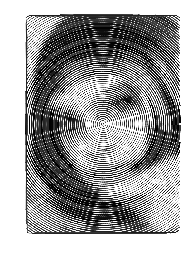
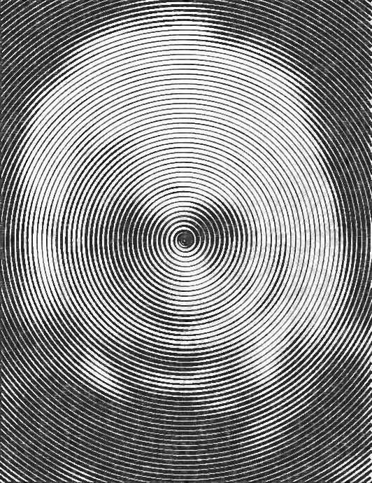
This is the basic functionality of the script. Some extra care has
been taken to skip some line segments that connects one edge of the
image and another. Some sample results are shown below.


