What is peak prominence?
In topography, prominence (also referred to as autonomous height, relative height, and shoulder drop in US English, and drop or relative height in British English) measures the height of a mountain or hill’s summit relative to the lowest contour line encircling it but containing no higher summit within it. It is a measure of the independence of a summit.
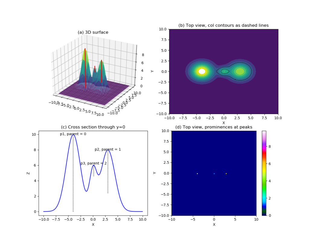
The following image gives an example of the peak prominence definition.
Figure 1a plots a 3D mesh surface with 3 local peaks. The red solid
vertical lines link the top most point of each peak and the
level of the encircling contour of the peak. From left to right, the
peaks are labeled as p1, p3 and p2 (following the order of their
heights). A contour representation of these 3 peaks are given in
Figure 1b, the bigger dashed black contour is the encircling contour of peak p2,
and the smaller one of peak p3. Cutting a vertical profile along
the central line of y=0 gives Figure 1c. Again the highest peak is
p1 on the left. Being the highest within this system, its parent is
labeled 0 (or no parent). p2 is the 2nd highest, with a parent peak
of p1, because it is enclosed by the encircling contour of p1 (not shown in Figure). p3 is the lowest one, with its
parent being p2, because its enclosed by the encircling contour of
p2 (the bigger dashed contour in Figure 1b). The last figure Figure 1d plots out the locations of the 3 peaks
in a top-down view, and the color of the 3 pixels represent their peak
prominence, i.e. the length of the vertical lines in Figure 1a and 1c.
Therefore, peak prominence measures the independence of a local peak,
or, how much a local peak stands out in relation to other local peaks
in the same mountain range. In the given sample, p1 is the dominant
peak, with no parent. The prominence of p1 is also its absolute
height (in this case, 9.8). p2 is a secondary peak with a
prominence of 5.4 and an absolute height of 7.8. Visually, it is a
relatively independent peak, with a prominence/height ratio of
5.4/7.8=0.69. In contrary, p3 is more of a local disturbance than
an independent peak, which could be explained by its low
prominence/height ratio (1.4/6.0=0.23).
What do I need peak prominence for?
I found the concept of peak prominence when I was searching for some
methods to identify and locate certain salient features in an
atmospheric variable. For instance, in the identification and
location of extra-tropical cyclones, such features could be a dome in
the field of the smoothed 850 hPa level relative vorticity, or a
dome in the inverted sea level pressure field. Extra-tropical cyclones
can appear as single core, or multi-core systems where a single
large low pressure system may enclose one or two smaller pressure
troughs in it, much like a upside-down version of Figure 1. This kind of
phenomenon actually happens rather frequently: about 25% of
extra-tropical cyclones experience at least one multi-core time point
in their life times. To identify such systems, one may need to make a
distinction between legitimate sub-cores in the pressure field from
those local disturbances that are nothing but noise in the data. Such
noise can be quite abundant in areas with complex terrain, such as
coastal regions, and will be more frequent in data with higher
horizontal resolution.
Peak prominence seems to be the ideal tool for this task. To
work with the pressure field one only needs to inverse the sign of the
pressure, so that low pressure centers become "peaks" in the inverted
pressure surface. An extra-tropical cyclone is required to have a peak
with some minimum height, and a multi-core cyclone should only be
labeled when its sub-core peaks are relatively "independent",
e.g. with a prominence/height ratio >=0.6. If a local peak’s
prominence/height ratio is too low, we could safely treat it as a
regional disturbance, and group it into its parent.
The filiation relationships of the peaks in a mountain range form a directed topological tree structure, which might be of importance in some applications.
How to find peak prominence?
I created a getPromience() function to compute the prominences of peaks in a 3D
surface. It’s too lengthy to post here, and you can download the
script file from this Github repo. The script comes with the same example as shown
in Figure 1. Only some important points are given below.
Peak prominences are found using a contouring approach. It makes a sequence of horizontal slides of the given 3D surface, starting from the highest to the lowest level:
for ii,levii in enumerate(levels[::-1]):
where levels is:
levels=np.arange(vmin,vmax+step,step).astype('float')
With vmin being the lowest level of the input 3D surface,
and vmax the maximum. levels is an evenly spaced height levels
with an interval of step. The process can be visualized as a big
flood that submerged all the peaks gradually retreats, creating bigger
and bigger "islands".
In the beginning, only the very tip of the highest peak gets revealed:
if len(peaks)==0:
	npeak+=1
	peaks[npeak]=[contjj,]
	prominence[npeak]=levii
	parents[npeak]=0
It is given an numerical id (npeak), and its location (contii)
recorded. Since it’s the highest peak, its prominence is the same as
the absolute value (levii), and its parent is 0.
Each time the sea level drops by a step, new coastal lines (contours) are created, and we examine which of them form an enclosing relationship with existing peaks:
match_list=[]
for kk,vv in peaks.items():
	if contjj.contains_path(vv[-1]):
		match_list.append(kk)
where kk is the numerical id for each peak, vv a list of contours for peak kk, starting from the smallest (highest) to the largest (lowest).
In such cases, we group the contours belonging to the same peak into a
single list. The prominence of a local peak that gets enclosed by a
contour that contains a higher peak is defined as the difference
between the height of its inner most contour (peaks[mm][0].level)
and the height of the contour that encloses the these peaks (levii):
if len(match_list)>1:
	match_heights=[peaks[mm][0].level for mm in match_list]
	max_idx=match_list[np.argmax(match_heights)]
	for mm in match_list:
		if prominence[mm]==peaks[mm][0].level and mm!=max_idx:
			prominence[mm]=peaks[mm][0].level-levii
			parents[mm]=max_idx
	peaks[max_idx].append(contjj)
If a newly emerging contour doesn’t enclose anything, it forms a new peak/island on its own:
if len(match_list)==0:
	npeak+=1
	peaks[npeak]=[contjj,]
	prominence[npeak]=levii
	parents[npeak]=0
This process repeats till the flood completely retreats and the sea
level drops to vmin. In the end, we get a collection of peaks,
each labeled with a numerical id, with all its contour levels from the
highest to the lowest. Prominence and parent id are also recorded.
The function calls matplotlib‘s contour(), or contourf()
function to compute the contour lines. contour() is used if it is
known beforehand that all contours are entirely included in the data
domain, and no contour touches the boundary of the map. Or, we know
such boundary-touching contours exist but decide to ignore them.
if not include_edge:
	conts=ax.contour(lons,lats,var,levels)
	contours=conts.collections[::-1]
	got_levels=conts.cvalues
	if not np.all(got_levels==levels):
		levels=got_levels
	ax.cla()
Alternatively,
contourf() is used so that unclosed contours are allowed:
if include_edge:
	csii=ax.contourf(lons,lats,var,[levii,vmax+step])
	csii=csii.collections[0]
	ax.cla()
Notice that contour() can obtain all contours across all levels in
one go, but contourf() has to be repeated for each level step.
The getPromience() function also offers some optional input
arguments that allow one to filter out some local peaks by their area
(min_area and max_area), or minimum height (min_depth). The area
of the peaks can be computed using latitude/longitude coordinates, and
measured in km^2, with the help of the Green’s
theorem.


