The goal
Mann-Kendall (MK) test is a non-parametric statistical test to validate the existence of monotonic upward/downward trend in a time series. The test is non-parametric, meaning that it does not assume the underlying distribution of the data being examined.
In the context of climatic researches, it can be used to examine the significance of, for example, the rising average temperature over a region during a certain period.
There are available Python implementations of the MK test, for instance, the pyMannKendall module, which is a much more versatile module than what we are going to build in this post.
However, when dealing with climatic/meteorological data, it is often desirable to perform not just one test on a single time series, but multiple tests on all of the grid cells within a domain. With increasing horizontal resolutions of datasets, this can be fairly slow if done using a nested for loop strategy in Python.
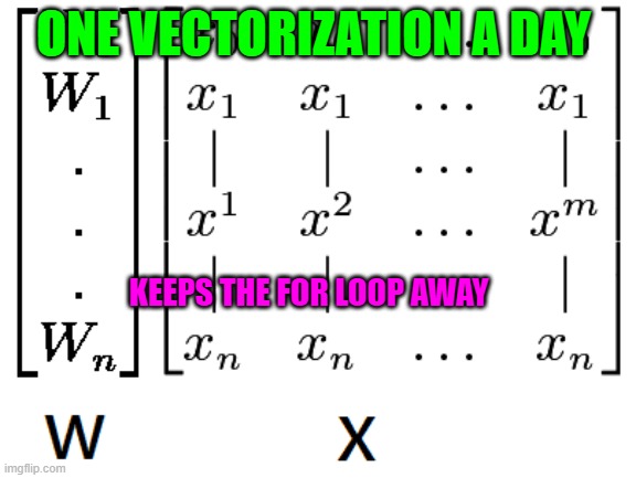
Therefore, in this post we are going to explore a vectorized Mann-Kendall trend test implementation that is designed to speed up such kind of computations.
The Mann-Kendall trend test
The computations in a MK test are:
1. Denote a 1-dimensional time series as \(x_1, x_2, \cdots, x_n\).
2. Determine the signs of all possible pairs of \(x_j – x_k\):
\[
s_{jk} = sgn(x_j – x_k) =
\left\{\begin{matrix}
1 & if\; x_j > x_k \\
0 & if\; x_j = x_k \\
-1 & if\; x_j < x_k \\
\end{matrix}\right.
\]
where \(j > k\), i.e. a later measurement minus an earlier one. It’s easy to work out that there are \(\frac{n(n-1)}{2}\) such pairs.
3. Sum up all the \(s_{jk}\):
\[
S = \sum_{k-1}^{n-1} \sum_{j-k+1}^{n} sgn(x_j – x_k)
\]
4. Compute the variance of \(S\):
\[
VAR(S) = \frac{1}{18} [n(n-1)(2n + 5) – T]
\]
where \(T\) is an adjustment factor for ties in the time series, and is computed as:
\[
T = \sum_{p-1}^g t_p (t_p – 1)(2t_p +5)
\]
where:
\(g\): the number of tied groups,
\(t_p\): the number of values in the group \(p\).
E.g. the sequence \(1, 2, 2, 9.3, -1, 9.3, 5, 7, 2\) has 3 tied groups:
(1) 2: appeared 3 times, giving \(t_1 = 3\).
(2) 9.3: appeared twice, giving \(t_2 = 2\).
Then the tie argument would be:
\[
T = \sum_{p-1}^g t_p (t_p – 1)(2t_p +5) = 3 \times (3 – 1) \times (2
\times 3 + 5) + 2 \times (2 – 1) \times (2 \times 2 + 5) = 84
\]
5. Compute the MK test statistic:
\[
Z = \left\{\begin{matrix}
\frac{S-1}{\sqrt{VAR(S)}} & if \; S > 0 \\
0 & if \, S = 0 \\
\frac{S+1}{\sqrt{VAR(S)}} & if \; S < 0
\end{matrix}\right.
\]
6. Do the hypothesis test using \(Z\) as the standard score on a standard Normal distribution.
More details of the algorithm can be found in this page.
Serial version
The serial version is relatively straightforward:
import numpy as np
from scipy.stats import norm

def countTies(data):
    '''Count the number of ties in each group for all groups
    '''
    counts = np.unique(data, return_counts=True)[1]
    counts = counts[np.where(counts>1)]
    if len(counts) == 0:
        return [0,]
    else:
        return counts

def MannKendallTrend(data, tails=2, verbose=True):
    '''Perform Mann-Kendall Trend test on a timeseries

    Args:
        data (ndarray): 1d array, time series to examine trend.
    Keyword Args:
        tails (int): 1 or 2, 1- or 2- tailed test.
    Returns:
        p (float): p-value of the test statistic.
    '''

    n = data.size
    s = np.sign(data[None,:] - data[:,None])
    s = np.triu(s).sum()

    # Count ties
    counts = countTies(data)
    tt = np.array(list(map(lambda x:x*(x-1)*(2*x+5), counts)))
    tt = np.sum(tt)

    var = (n*(n-1)*(2*n+5)-tt)/18.
    z = (s - np.sign(s)) / np.sqrt(var)
    p = norm.cdf(z)
    p = 1-p if p>0.5 else p

    if tails == 2:
        p = p*2

    if verbose:
        print('\n# <testwmw>: s',s)
        print('# <testwmw>: counts',counts)
        print('# <testwmw>: tt',tt)
        print('# <testwmw>: var',var)
        print('# <testwmw>: z',z)
        print('# <testwmw>: p',p)

    return p
The function MannKendallTrend() first computes the signs of all
possible pairs using
s = np.sign(data[None,:] - data[:,None])
Note that this is already using some vectorization trick rather than a nested for loop. Then the signs are summed using:
s = np.triu(s).sum()
This is taking the upper triangle of the s matrix, and we are not
excluding cases of j = k on the diagonal line, since their
contributions would be 0 anyways.
Then the tied values are found using the countTies() function, and
the tie adjustment factor computed.
Lastly, the percentile of a standard Normal distribution is obtained
using the scipy.stats.norm.cdf() function. The p-value is doubled
if a 2-tailed test is desired.
Vectorized version
1st implementation
The vectorized version will follow generally the same procedures as the serial version. The trickiest part lies in the computation of the tie adjustment factor.
To simply things, we are assuming the input data to be a 2D array,
with shape (m, n), where m is the number of records, and n the
dimension size of each record.
For a multi-cell trend analysis using climatic data, n would be the
length of the time series in each grid cell, and m the total number of
grid cells in the data. Therefore, if the data come in as a 3D cube
with the format of (time, latitude, longitude), one would
need to reshape it into (latitude * longitude, time).
The 1st vectorized version I wrote is the following:
def MannKendallTrend2D(data, tails=2, axis=0, verbose=True):
    '''Vectorized Mann-Kendall tests on 2D matrix rows/columns

    Args:
        data (ndarray): 2d array with shape (m, n).
    Keyword Args:
        tails (int): 1 for 1-tail, 2 for 2-tail test.
        axis (int): 0: test trend in each column. 1: test trend in each
            row.
    Returns:
        z (ndarray): If <axis> = 0, 1d array with length <n>, standard scores
            corresponding to data in each row in <x>.
            If <axis> = 1, 1d array with length <m>, standard scores
            corresponding to data in each column in <x>.
        p (ndarray): p-values corresponding to <z>.
    '''

    if np.ndim(data) != 2:
        raise Exception("<data> should be 2D.")

    # alway put records in rows and do M-K test on each row
    if axis == 0:
        data = data.T

    m, n = data.shape
    mask = np.triu(np.ones([n, n])).astype('int')
    mask = np.repeat(mask[None,...], m, axis=0)
    s = np.sign(data[:,None,:]-data[:,:,None]).astype('int')
    s = (s * mask).sum(axis=(1,2))

    #--------------------Count ties--------------------
    counts = countTies(data)
    tt = counts * (counts - 1) * (2*counts + 5)
    tt = tt.sum(axis=1)

    #-----------------Sample Gaussian-----------------
    var = (n * (n-1) * (2*n+5) - tt) / 18.
    eps = 1e-8  # avoid dividing 0
    z = (s - np.sign(s)) / (np.sqrt(var) + eps)
    p = norm.cdf(z)
    p = np.where(p>0.5, 1-p, p)

    if tails==2:
        p=p*2

    return z, p
Note that:
Although an axis argument is provided to allow specifying the
axis of the time dimension, I’m forcing the data to be in the (m, n) layout as mentioned above, by doing a transpose if axis=0:
data = data.T.
The signs of all possible pairs are computed using:
s = np.sign(data[:,None,:]-data[:,:,None]).astype('int')
This is similar to the serial version except that it handles all grid cells simultaneously.
Again, we take only the upper triangle and sum it up:
mask = np.triu(np.ones([n, n])).astype('int')
mask = np.repeat(mask[None,...], m, axis=0)
s = np.sign(data[:,None,:]-data[:,:,None]).astype('int')
s = (s * mask).sum(axis=(1,2))
The tied groups are obtained using a new countTies() function, given
below:
def countTies(x):
    '''Count number of ties in rows of a 2D matrix

    Args:
        x (ndarray): 2d matrix.
    Returns:
        result (ndarray): 2d matrix with same shape as <x>. In each
            row, the number of ties are inserted at (not really) arbitary
            locations.
            The locations of tie numbers in are not important, since
            they will be subsequently put into a formula of sum(t*(t-1)*(2t+5)).

    Inspired by: https://stackoverflow.com/a/24892274/2005415.
    '''
    if np.ndim(x) != 2:
        raise Exception("<x> should be 2D.")

    m, n = x.shape
    pad0 = np.zeros([m, 1]).astype('int')

    x = copy.deepcopy(x)
    x.sort(axis=1)
    diff = np.diff(x, axis=1)

    cated = np.concatenate([pad0, np.where(diff==0, 1, 0), pad0], axis=1)
    absdiff = np.abs(np.diff(cated, axis=1))

    rows, cols = np.where(absdiff==1)
    rows = rows.reshape(-1, 2)[:, 0]
    cols = cols.reshape(-1, 2)
    counts = np.diff(cols, axis=1)+1
    result = np.zeros(x.shape).astype('int')
    result[rows, cols[:,1]] = counts.flatten()

    return result
This part is a bit tricky to vectorize, because the number of ties would be in general different for each record.
For instance, the 1st record (now has been forced to be the 1st row in
data), contains 3 groups of ties:
\[
t_1 = 2; \; t_2 = 2; \; t_3 = 3
\]
If we put that in an array, it would be [2, 2, 3], or [2, 3, 2], since ordering doesn’t really matter.
Suppose the 2nd record (2nd row in data) has 1 group of ties with 2
values, then the output array for that would be [2, ].
The 3rd record may have no ties, giving [].
Therefore, the vectorized tie-counts array would have different number of values in its rows.
The solution would be to pad 0s to make it a squared shape, and the
size to pad to can be just the length of the time series n, since it
is guaranteed that the number of tie groups in a n-length time series
is always smaller than n.
Zero-padding is acceptable, because it is observed that these padded 0s make no contribution to the final result, since the formula we use to compute tie adjustment is
tt = counts * (counts - 1) * (2*counts + 5)
Additionally, the positions of tie counts do not matter, since they
are latter summed up in tt = tt.sum(axis=1).
So, the basic idea of countTies() is:
- make a deep copy of the input
data, because we are going to sort the data in order along the time dimension (x.sort(axis=1)). - after sorting, compute the differences between consecutive pairs.
- 0 in the differentiated consecutive pairs denotes a tie, and multiple consecutive 0s denote a tie group with more than 2 tied values.
- replace such 0s with 1s, and all other places with 0s.
- find the boundaries of such 1s, and they encode the indices of the tied values.
- the number of ties in each group can be worked out using these indices, and these tie counts are put to the locations of the last tied values.
- these are all done in a vectorized manner.
In the end, the resultant result variable is a (m, n) array. In
each row, the number of ties in different tie groups in that row are
inserted at different places (recall that positions are
insignificant), and all other places are filled with 0s (recall that
0s do not contribute).
With the tie adjustment factor worked out, the rest of the
MannKendallTrend2D() function is fairly self-explanatory.
This version works pretty well already. I tested it on a sample case
with the input data being (50, 145, 192) in size (in (time, latitude, longitude) layout). On my desktop it took about 1.28
seconds. This solution was also offered as
Stackoverflow answer.
2nd implementation
One big issue with the above implementation is memory usage. With
vectorization speed gain we are sacrificing memory efficiency. For larger
sized data, I got overflow warning and numpy simply refused to
compute.
The biggest RAM eating block lies here:
mask = np.triu(np.ones([n, n])).astype('int')
mask = np.repeat(mask[None,...], m, axis=0)
s = np.sign(data[:,None,:]-data[:,:,None]).astype('int')
namely, the vectorized computation of all the pair-wise differences.
It is noticed that we don’t really need the complete matrix of
data[:,None,:] - data[:,:,None], since only the upper triangle is
needed, and the lower triangle gives only the opposite values.
Therefore I came up with this 2nd version (the countTies() function
stays the same):
def MannKendallTrend2D(data, tails=2, axis=0, verbose=True):
    '''Vectorized Mann-Kendall tests on 2D matrix rows/columns

    Args:
        data (ndarray): ndarray with shape (m, n).
    Keyword Args:
        tails (int): 1 for 1-tail, 2 for 2-tail test.
        axis (int): 0: test trend in each column. 1: test trend in each
            row.
    Returns:
        z (ndarray): If <axis> = 0, 1d array with length <n>, standard scores
            corresponding to data in each row in <x>.
            If <axis> = 1, 1d array with length <m>, standard scores
            corresponding to data in each column in <x>.
        p (ndarray): p-values corresponding to <z>.
    '''

    if np.ndim(data) != 2:
        raise Exception("<data> should be 2D.")

    # alway put records in rows and do M-K test on each row
    if axis == 0:
        data = data.T

    m, n = data.shape
    mask = np.triu_indices(n, 1)
    s = np.sign(data[:,mask[1]] - data[:,mask[0]]).sum(axis=1)

    #--------------------Count ties--------------------
    counts = countTies(data)

    tt = counts * (counts - 1) * (2*counts + 5)
    tt = tt.sum(axis=1)

    #-----------------Sample Gaussian-----------------
    var = (n * (n-1) * (2*n+5) - tt) / 18.
    eps = 1e-8  # avoid dividing 0
    z = (s - np.sign(s)) / (np.sqrt(var) + eps)
    p = norm.cdf(z)

    p = np.where(p>0.5, 1-p, p)

    if tails==2:
        p=p*2

    return z, p
To highlight the differences, these are the new lines computing the pair-wise differences and signs:
mask = np.triu_indices(n, 1)
s = np.sign(data[:,mask[1]] - data[:,mask[0]]).sum(axis=1)
The np.triu_indices() gives indices of the upper triangle, so we can
save half of original memory.
3rd implementation
Unfortunately, it is still quite heavy on RAM usage.
My 3rd attempt is no longer strictly vectorized, but a compromise
between fully vectorized computation and an iterated one. I could not
figure out an efficient solution using tools in numpy or scipy for
this, and I think it might be a good place to look for other directions
like cython or compiled code.
The 3rd MannKendallTrend2D() is:
def MannKendallTrend2D(data, tails=2, axis=0, verbose=True):
    '''Vectorized Mann-Kendall tests on 2D matrix rows/columns

    Args:
        data (ndarray): ndarray with shape (m, n).
    Keyword Args:
        tails (int): 1 for 1-tail, 2 for 2-tail test.
        axis (int): 0: test trend in each column. 1: test trend in each
            row.
    Returns:
        z (ndarray): If <axis> = 0, 1d array with length <n>, standard scores
            corresponding to data in each row in <x>.
            If <axis> = 1, 1d array with length <m>, standard scores
            corresponding to data in each column in <x>.
        p (ndarray): p-values corresponding to <z>.
    '''

    if np.ndim(data) != 2:
        raise Exception("<data> should be 2D.")

    # alway put records in rows and do M-K test on each row
    if axis == 0:
        data = data.T

    m, n = data.shape
    mask = np.triu_indices(n, 1)
    try:
        s = np.sign(data[:,mask[1]] - data[:,mask[0]]).sum(axis=1)
    except MemoryError:
        # data size too big, do it in batches
        i = 1
        s = np.zeros(m)
        while True:
            k = m//(n*i)
            t = m//k + 1
            try:
                for j in range(t):
                    id1 = j*k
                    id2 = min((j+1)*k, m)
                    sj = np.sign(data[id1:id2,mask[1]] - data[id1:id2,mask[0]]).sum(axis=1)
                    s[id1:id2] = sj
            except:
                i +=1
            else:
                break

    #--------------------Count ties--------------------
    counts = countTies(data)

    tt = counts * (counts - 1) * (2*counts + 5)
    tt = tt.sum(axis=1)

    #-----------------Sample Gaussian-----------------
    var = (n * (n-1) * (2*n+5) - tt) / 18.
    eps = 1e-8  # avoid dividing 0
    z = (s - np.sign(s)) / (np.sqrt(var) + eps)
    p = norm.cdf(z)

    p = np.where(p>0.5, 1-p, p)

    if tails==2:
        p=p*2

    return z, p
The new part is:
mask = np.triu_indices(n, 1)
try:
    s = np.sign(data[:,mask[1]] - data[:,mask[0]]).sum(axis=1)
except MemoryError:
    # data size too big, do it in batches
    i = 1
    s = np.zeros(m)
    while True:
        k = m//(n*i)
        t = m//k + 1
        try:
            for j in range(t):
                id1 = j*k
                id2 = min((j+1)*k, m)
                sj = np.sign(data[id1:id2,mask[1]] - data[id1:id2,mask[0]]).sum(axis=1)
                s[id1:id2] = sj
        except:
            i +=1
        else:
            break
So I’m trying in a try block the half-memory solution in the 2nd
implementation to see if there is enough RAM to handle it. If not, I
divide the entire task into a number of chunks, each time using the
half-memory upper triangle trick on the chunk only, and put together the
final array s piece-by-piece. This has been proven to work for
big sized data that were giving me RAM overflow using the fully
vectorized version.
Summary
In this post, I shared a vectorized Mann-Kendall trend test using
numpy and scipy. It is helpful to carry out multiple trend tests
on a gridded dataset, and can be considerably faster than using a
nested for loop. However, it achieves this speed-up by sacrificing
memory efficiency, and may trigger a RAM overflow on large data size.


