
The goal
In previous posts we’ve talked about how to
- Create a simple neural network.
- Perform 2D and 3D convolutions.
- Perform 2D and 3D pooling.
- Perform back-propagation in a convolution layer.
all with numpy implementations.
With these building blocks, we can implement a convolutional neural network (CNN) from scratch. This is the topic of this post. Specifically, we will cover:
- How to combine the building blocks we have had to create a simple CNN with convolution layers, pooling layers and fully-connected layers.
- A serial implementation of CNN using
numpy. - A vectorized implementation of CNN using
numpy. - Use the vectorized CNN to classify hand-written images from the MNIST dataset.
Design choice and notations
Class design
Similar to the implementation of the multi-layer neural network (see this post), we are going to wrap up the CNN implementation in a Class.
Since we have got all the basic building blocks — 2D and 3D convolution functions with back-propagation, 2D and 3D pooling functions and fully connected neural network layers — it would make sense to design our CNN class in a way that allows flexible designs of the network, such that one can plugin these building blocks like lego pieces to form networks with different architectures. For instance, suppose the we are building a CNN that has:
- 1 convolution layer at the beginning, followed by
- 1 pooling layer, followed by
- another convolution layer, and finally
- 2 fully connected layers.
The code for creating such a CNN may look like something like this:
cnn = CNNClassifier(...)

layer1 = ConvLayer(...)
layer2 = PoolLayer(...)
layer3 = ConvLayer(...)
layer4 = FlattenLayer(...)
layer5 = FCLayer(...)
layer6 = FCLayer(...)

cnn.add(layer1)
cnn.add(layer2)
cnn.add(layer3)
cnn.add(layer4)
cnn.add(layer5)
cnn.add(layer6)
Therefore, we need to implement these classes:
ConvLayer: the 2D/3D convolution layer class.PoolLayer: the pooling layer class.FcLayer: the fully connected layer class.CNNClassifier: the classifier CNN class.
Note that I’ve added an additional FlattenLayer class that
does nothing but reshapes the outputs from convolution/pooling layers
into a vector, for it to be later processed by the subsequent
fully-connected layers.
Inside the CNNClassifier, each iteration of the training process
would just do a for loop over the building block layers, and pass
the data forward from one layer to another. During the
back-propagation stage, the errors are passed between layers in the
reversed order.
To achieve such a structure, we need to write our building block layer classes with a unified interface. Taking into account the workflow inside a CNN (more details in later section), these layers should have these methods:
init(): perform some initialization tasks in the layer.forward(): take the input into the layer, do the computations, and return the weighted sums (\(Z^{(l)}\)) and activations (\(a^{(l)}\)) of the current layer.backPropError(): take the error term (\(\delta^{(l)}\)) coming from the next layer, and back-propagate to get the error term for the previous layer (\(\delta^{(l-1)}\)).computeGradient(): compute the gradients of the parameters in the current layer wrt to the loss function (\(\partial J / \partial w^{(l)}\)), and the gradients of the bias terms (\(\partial J / \partial b^{(l)}\)).gradientDescent(): given the gradients computed from thecomputeGradient()method, perform gradient descent parameter update.
Note that some of these methods are not meaningful for some of the
layers types. For instance, there are no trainable parameters in a
pooling layer, so PoolLayer does not need to do anything in
its computeGradient() and gradientDescent() methods. Similar for
FlattenLayer. The table below summarizes what computations are
actually done in these methods for different layer types.
| Method/Layer type | ConvLayer / FCLayer | PoolLayer | FlattenLayer |
|---|---|---|---|
init() |
randomly initialize parameters and biases | N\A | N\A |
forward() |
compute weighted sum, add bias and compute activation function | pooling | flatten each input to an 1D array |
backPropError() |
back-prop the errors | unpooling | reshape each input to its original shape |
computeGradient() |
compute the parameter/bias gradients | N\A | N\A |
gradientDescent() |
gradient descent update | N\A | N\A |
We have covered all the computations in Table 1 in previous posts (see create a simple neural network, perform 2D and 3D convolutions, perform 2D and 3D pooling, perform back-propagation in a convolution layer).
To put everything together, it would be helpful to do a recap on the notations.
Notations
For a convolution layer which is layer l in the CNN:
- \(f^{(l)}\): height and width of the convolution kernel/filter.
- \(p^{(l)}\): padding applied before convolution.
- \(s^{(l)}\): stride applied during convolution.
- \(n^{(l)}_c\): number of filters in the convolution layer.
- \(n^{(l-1)}_H \times n^{(l-1)}_W \times n^{(l-1)}_c\): size of the input to the convolution layer, i.e. activation of layer \(l-1\), as the product of height (\(n^{(l-1)}_H\)), width (\(n^{(l-1)}_W\)) and number of channels (\(n^{(l-1)}_c\)).
- \(n^{(l)}_H \times n^{(l)}_W \times n^{(l)}_c\): size of the output of the convolution layer.
- \(w^{(l,k)}\): the kth convolution kernel/filter of layer \(l\): \(w^{(l,k)} \in \mathbb{R}^{f^{(l)} \times f^{(l)}}\).
- \(z^{(l,k)}\): convolution result from the kth filter: \(z^{(l,k)} \in \mathbb{R}^{n^{(l)}_H \times n^{(l)}_W}\).
- \(z^{(l)}\): stacked convolution results from all filters: \(z^{(l)} \in \mathbb{R}^{n^{(l)}_H \times n^{(l)}_W \times n^{(l)}_c}\).
- \(b^{(l, k)}\): bias term for the kth filter in the layer: \(b^{(l,k)} \in \mathbb{R}\).
- \(b^{(l)}\): bias term for all the filters in the layer: \(b^{(l)} \in \mathbb{R}^{n^{(l)}_c}\).
- \(a^{(l,k)}\): result of the activation function for the kth filter in the layer: \(a^{(l, k)} \in \mathbb{R}^{n^{(l)}_H \times n^{(l)}_W}\).
- \(a^{(l)}\): result of the activation function for all the filters in the layer: \(a^{(l)} \in \mathbb{R}^{n^{(l)}_H \times n^{(l)}_W \times n^{(l)}_c}\).
For a pooling layer which is layer \(l\) in the CNN:
- \(f^{(l)}\): height and width of the pooling kernel/filter.
- \(p^{(l)}\): padding applied before pooling.
- \(s^{(l)}\): stride applied during pooling.
For a fully connected layer which is layer \(l\) in the CNN:
- \(s_l\): number of neurons in the layer.
- \(\theta^{(l)}\): weight matrix of the layer.
- \(b^{(l)}\): bias term in the layer.
- \(z^{(l)}\): weighted sum.
- \(a^{(l)}\): activation of the layer.
Additional design choices
To simplify the CNN implementation, we are also making these following design choices:
-
Assume all training data and convolution filters to have square shapes (height equals width).
-
Use ReLU as the activation function for all hidden convolution and hidden fully connected layers.
-
Use softmax as the activation function of the last layer.
-
Use HE initialization (see later for details) for convolution and fully connected layers.
-
Use max-pooling for pooling layers.
-
Do a default
[-0.5, 0.5]clipping on the weights in convolution and fully connected layers. -
Do a l2 regularization on the parameters (excluding bias terms) of convolution and fully connected layers.
-
Batch normalization and dropout are not implemented.
Computations in a CNN – forward propagation
To help make the explanations more concrete, suppose that the CNN we are building has the following structure:
- Input. Recall that the MNIST dataset consists of gray-scale images with dimensions of \(28 \times 28 \times 1\).
- 1 convolution layer with \(f^{(1)} = 3\), \(p^{(1)} = 0\), \(s^{(1)} = 1\) and \(n_c^{(1)} = 10\). The output from this layer has shape \(26 \times 26 \times 10\).
- 1 pooling layer with \(f^{(2)} = 2\), \(p^{(2)} = 0\), \(s^{(2)} = 2\). The output from this layer has shape \(13 \times 13 \times 10\).
- another convolution layer with \(f^{(3)} = 5\), \(p^{(2)} = 0\), \(s^{(3)} = 1\), and \(n^{(3)}_c = 16\). The output from this layer has shape \(9 \times 9 \times 16\).
- a flatten layer to flatten the outputs from previous layer into shape \(1296 \times 1\).
- 1 fully connected layer with \(\theta^{(5)} \in \mathbb{R}^{100 \times 1296}\), i.e. the layer takes 1296 inputs and outputs 100 units.
- another fully connected layer with \(\theta^{(6)} \in \mathbb{R}^{10 \times100}\), i.e. the layer takes 100 inputs and outputs 10 units.
With the above CNN structure, for any training sample \(X^{(i)} \in \mathbb{R}^{28 \times 28 \times 1}\), the forward computation involves the following (see Figure 1 for illustration):
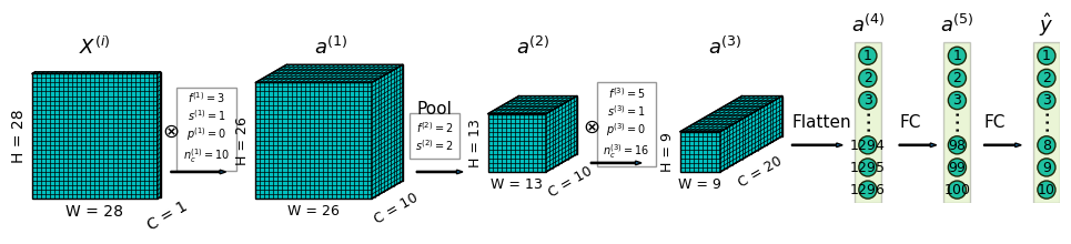
- In the 1st convolution layer, we have \(a^{(1)} = ReLU(z^{(1)} + b^{(1)}) = ReLU(w^{(1)} \otimes X^{(i)} + b^{(1)})\). Where \(\otimes\) is convolution operator, \(w^{(1)}\) is the convolution filter in layer \(1\). The activation \(a^{(1)}\) of each convolution layer has a shape of \(26 \times 26 \times 1\). After stacking up outputs from all 10 filters, output from the 1st convolution layer has a shape of \(26 \times 26 \times 10\).
- In the 2nd layer, max-pooling is performed with a filter size of 2 and a stride of 2, independently for each channel. Therefore the output has a shape of \(13 \times 13 \times 10\).
- In the 3rd layer, we have \(a^{(3)} = ReLU(z^{(3)} + b^{(3)}) = ReLU(w^{(3)} \otimes a^{(2)} + b^{(3)})\). The activation \(a^{(3)}\) of each convolution layer has a shape of \(9 \times 9 \times 1\), after stacking up outputs from all 16 filters, output from this convolution layer has a shape of \(9 \times 9 \times 16\).
- The 4th layer flattens the outputs from previous layer into shape \(1296 \times 1\).
- In the 5th layer, we have \(a^{(5)} = ReLU(z^{(5)} + b^{(5)}) = ReLU(\theta^{(5)} \cdot a^{(4)} + b^{(5)})\).
- In the 6th layer, we have \(\hat{y} = a^{(6)} = softmax(z^{(6)} + b^{(6)}) = ReLU(\theta^{(6)} \cdot a^{(5)} + b^{(6)})\). Note that we are using the softmax function as the last activation function.
Computations in a CNN – backward propagation
For each training sample (\(X^{(i)}\), \(y^{(i)}\)), we have a predicted output \(\hat{y}^{(i)}\), and a corresponding model error \(\hat{y}^{(i)} – y^{(i)}\). In order to update the model, we need to propagate this error backwards through the network.
The error back-propagation in fully connected layer is given as (see this post for more details):
\[
\delta^{(l-1)} = \theta^{(l)^T} \cdot \delta^{(l)} \odot g'(z^{(l-1)})
\]
The weight gradients are computed as:
\[
\frac{\partial J}{\partial \theta^{(l)}} = \delta^{(l)} \cdot a^{(l-1)^T}
\]
The bias gradients are computed as:
\[
\frac{\partial J}{\partial b^{(l)}} = \delta^{(l)}
\]
The error back-propagation in a max-pooling layer is simply assigning the error values back to the locations where the maxima values were during the pooling stage. And there are no trainable parameters in a pooling layer. (see this post for more details.)
The error back-propagation in convolution layer is given as (see this post for more details):
\[
\delta^{(l-1)} = \sum_{k=1}^{n^{(l)}_c} [ \delta^{(l,k)} \otimes_f Rot_{180}(w^{(l,k)}) \odot g'(z^{(l-1)})]
\]
The weight gradients are computed as:
\[
\frac{\partial J}{\partial w^{(l, k)}} = a^{(l-1)} \otimes
\delta^{(l,k)}, \; k=1,2,\cdots,n^{(l)}_c
\]
The bias gradients are computed as:
\[
\frac{\partial J}{\partial b^{(l,k)}} = \sum_i \sum_j \frac{\partial J}{\partial z^{(l,k)}_{i,j}} \frac{\partial z^{(l,k)}_{i,j}}{\partial b^{(l,k)}} = \sum_i \sum_j \delta^{(l,k)}_{i,j}
\]
numpy implementation – serial version
This section gives the serial version of the CNN implementation, that is, the training functions process 1 sample at a time. One vectorized version where training processes multiple samples at a time is given in the next section.
ConvLayer
Code first:
class ConvLayer(object):
    def __init__(self, f, pad, stride, nc_in, nc, learning_rate, af=None, lam=0.01,
            clipvalue=0.5):
        '''Convolutional layer

        Args:
            f (int): kernel size for height and width.
            pad (int): padding on each edge.
            stride (int): convolution stride.
            nc_in (int): number of channels from input layer.
            nc (int): number of channels this layer.
            learning_rate (float): initial learning rate.
        Keyword Args:
            af (callable): activation function. Default to ReLU.
            lam (float): regularization parameter.
            clipvalue (float): clip gradients within [-clipvalue, clipvalue]
                during back-propagation.

        The layer has <nc> channels/filters. Each filter has shape (f, f, nc_in).
        The <nc> filters are saved in a list `self.filters`, therefore `self.filters[0]`
        corresponds to the 1st filter.

        Bias is saved in `self.biases`, which is a 1d array of length <nc>.
        '''

        self.type = 'conv'
        self.f = f
        self.pad = pad
        self.stride = stride
        self.lr = learning_rate
        self.nc_in = nc_in
        self.nc = nc
        if af is None:
            self.af = ReLU
        else:
            self.af = af
        self.lam = lam
        self.clipvalue = clipvalue

        self.init()

    def init(self):
        '''Initialize weights

        Default to use HE initialization:
            w ~ N(0, std)
            std = \sqrt{2 / n}
        where n is the number of inputs
        '''
        np.random.seed(100)
        std = np.sqrt(2/self.f**2/self.nc_in)
        self.filters = np.array([
            np.random.normal(0, scale=std, size=[self.f, self.f, self.nc_in])
            for i in range(self.nc)])
        self.biases = np.random.normal(0, std, size=self.nc)

    @property
    def n_params(self):
        '''Number of parameters in layer'''
        n_filters = self.filters.size
        n_biases = self.nc
        return n_filters + n_biases

    def forward(self, x):
        '''Forward pass of a single image input'''

        x = force3D(x)
        x = padArray(x, self.pad, self.pad)
        # input size:
        ny, nx, nc = x.shape
        # output size:
        oy = (ny+2*self.pad-self.f)//self.stride + 1
        ox = (nx+2*self.pad-self.f)//self.stride + 1
        oc = self.nc
        weight_sums = np.zeros([oy, ox, oc])

        # loop through filters
        for ii in range(oc):
            slabii = conv3D3(x, self.filters[ii], stride=self.stride, pad=0)
            weight_sums[:, :, ii] = slabii[:, :]

        # add bias
        weight_sums = weight_sums+self.biases
        # activate func
        activations = self.af(weight_sums)

        return weight_sums, activations

    def backPropError(self, delta_in, z):
        '''Back-propagate errors

        Args:
            delta_in (ndarray): delta from the next layer in the network.
            z (ndarray): weighted sum of the current layer.
        Returns:
            result (ndarray): delta of the current layer.

        The theoretical equation for error back-propagation is:

            \delta^{(l)} = \delta^{(l+1)} \bigotimes_f Rot(W^{(l+1)}) \bigodot f'(z^{(l)})

        where:
            \delta^{(l)} : error of layer l, defined as \partial J / \partial z^{(l)}.
            \bigotimes_f : convolution in full mode.
            Rot() : is rotating the filter by 180 degrees, i.e. a kernel flip.
            W^{(l+1)} : weights of layer l+1.
            \bigodot : Hadamard (elementwise) product.
            f() : activation function of layer l.
            z^{(l)} : weighted sum in layer l.

        Computation in practice is more complicated than the above equation.
        '''

        # number of channels of input to layer l weights
        nc_pre = z.shape[-1]
        # number of channels of output from layer l weights
        nc_next = delta_in.shape[-1]

        result = np.zeros_like(z)
        # loop through channels in layer l
        for ii in range(nc_next):
            # flip the kernel
            kii = self.filters[ii, ::-1, ::-1, ...]
            deltaii = delta_in[:, :, ii]
            # loop through channels of input
            for jj in range(nc_pre):
                slabij = fullConv3D(deltaii, kii[:, :, jj], self.stride)
                result[:, :, jj] += slabij

        result = result*dReLU(z)

        return result

    def computeGradients(self, delta, act):
        '''Compute gradients of cost wrt filter weights

        Args:
            delta (ndarray): errors in filter ouputs.
            act (ndarray): activations fed into filter.
        Returns:
            grads (ndarray): gradients of filter weights.
            grads_bias (ndarray): 1d array, gradients of biases.

        The theoretical equation of gradients of filter weights is:

            \partial J / \partial W^{(l)} = a^{(l-1)} \bigotimes \delta^{(l)}

        where:
            J : cost function of network.
            W^{(l)} : weights in filter.
            a^{(l-1)} : activations fed into filter.
            \bigotimes : convolution in valid mode.
            \delta^{(l)} : errors in the outputs from the filter.

        Computation in practice is more complicated than the above equation.
        '''

        nc_out = delta.shape[-1]   # number of channels in outputs
        nc_in = act.shape[-1]      # number of channels in inputs

        grads = np.zeros_like(self.filters)

        for ii in range(nc_out):
            deltaii = np.take(delta, ii, axis=-1)
            gii = grads[ii]
            for jj in range(nc_in):
                actjj = act[:, :, jj]
                gij = conv3D3(actjj, deltaii, stride=1, pad=0)
                gii[:, :, jj] += gij
            grads[ii] = gii

        # gradient clip
        gii = np.clip(gii, -self.clipvalue, self.clipvalue)
        grads_bias = np.sum(delta, axis=(0, 1))  # 1d

        return grads, grads_bias

    def gradientDescent(self, grads, grads_bias, m):
        '''Gradient descent weight and bias update'''

        self.filters = self.filters * (1 - self.lr * self.lam/m) - self.lr * grads/m
        self.biases = self.biases-self.lr*grads_bias/m

        return
A few things to note:
- The
init()method uses HE initialization to initialize filters and biases. - The
forward()method uses the serial version of theconv3D3()function introduced in this post. - The
backPropError()method uses the serial version of thefullConv3D()function introduced in this post. - More details on the
computeGradients()method has been given in this post as well. - Computed weight gradients are clipped within the range of
[-self.clipvalue, self.clipvalue], to avoid exploding gradients. - In the
gradientDescent()method, the regularization term has been included inself.filters * (1 - self.lr * self.lam/m), whereself.lamis the regularization parameter.
PoolLayer
Code first:
class PoolLayer(object):
    def __init__(self, f, pad, stride, method='max'):
        '''Pooling layer

        Args:
            f (int): kernel size for height and width.
            pad (int): padding on each edge.
            stride (int): pooling stride. Required to be the same as <f>, i.e.
                non-overlapping pooling.
        Keyword Args:
            method (str): pooling method. 'max' for max-pooling.
                'mean' for average-pooling.
        '''

        self.type = 'pool'
        self.f = f
        self.pad = pad
        self.stride = stride
        self.method = method

        if method != 'max':
            raise Exception("Method %s not implemented" % method)

        if self.f != self.stride:
            raise Exception("Use equal <f> and <stride>.")

    @property
    def n_params(self):
        return 0

    def forward(self, x):
        '''Forward pass'''

        x = force3D(x)
        result, max_pos = poolingOverlap(x, self.f, stride=self.stride,
            method=self.method, pad=False, return_max_pos=True)
        self.max_pos = max_pos  # record max locations

        return result, result

    def backPropError(self, delta_in, z):
        '''Back-propagate errors

        Args:
            delta_in (ndarray): delta from the next layer in the network.
            z (ndarray): weighted sum of the current layer.
        Returns:
            result (ndarray): delta of the current layer.

        For max-pooling, each error in <delta_in> is assigned to where it came
        from in the input layer, and other units get 0 error. This is achieved
        with the help of recorded maximum value locations.

        For average-pooling, the error in <delta_in> is divided by the kernel
        size and assigned to the whole pooling block, i.e. even distribution
        of the errors.
        '''

        result = unpooling(delta_in, self.max_pos, z.shape, self.stride)
        return result
A few things to note:
- Only max-pooling is implemented.
- The
forward()methods uses the serial version of thepoolingOverlap()function, and thebackPropError()method uses the serial version of theunpooling()function, both introduced in this post. - As mentioned above, pooling layer has no trainable parameters and we
don’t need to implement the
gradientDescent()andcomputeGradients()methods.
FlattenLayer
Code first:
class FlattenLayer(object):
    def __init__(self, input_shape):
        '''Flatten layer'''

        self.type = 'flatten'
        self.input_shape = input_shape

    @property
    def n_params(self):
        return 0

    def forward(self, x):
        '''Forward pass'''

        x = x.flatten()
        return x, x

    def backPropError(self, delta_in, z):
        '''Back-propagate errors
        '''

        result = np.reshape(delta_in, tuple(self.input_shape))
        return result
This class is quite simple and self-explanatory.
FCLayer
Code first:
class FCLayer(object):

    def __init__(self, n_inputs, n_outputs, learning_rate, af=None, lam=0.01,
            clipvalue=0.5):
        '''Fully-connected layer

        Args:
            n_inputs (int): number of inputs.
            n_outputs (int): number of layer outputs.
            learning_rate (float): initial learning rate.
        Keyword Args:
            af (callable): activation function. Default to ReLU.
            lam (float): regularization parameter.
            clipvalue (float): clip gradients within [-clipvalue, clipvalue]
                during back-propagation.
        '''

        self.type = 'fc'
        self.n_inputs = n_inputs
        self.n_outputs = n_outputs
        self.lr = learning_rate
        self.clipvalue = clipvalue

        if af is None:
            self.af = ReLU
        else:
            self.af = af

        self.lam = lam   # regularization parameter
        self.init()

    @property
    def n_params(self):
        return self.n_inputs*self.n_outputs + self.n_outputs

    def init(self):
        '''Initialize weights

        Default to use HE initialization:
            w ~ N(0, std)
            std = \sqrt{2 / n}
        where n is the number of inputs
        '''
        std = np.sqrt(2/self.n_inputs)
        np.random.seed(100)
        self.weights = np.random.normal(0, std, size=[self.n_outputs, self.n_inputs])
        self.biases = np.random.normal(0, std, size=self.n_outputs)

    def forward(self, x):
        '''Forward pass'''

        z = np.dot(self.weights, x)+self.biases
        a = self.af(z)

        return z, a

    def backPropError(self, delta_in, z):
        '''Back-propagate errors

        Args:
            delta_in (ndarray): delta from the next layer in the network.
            z (ndarray): weighted sum of the current layer.
        Returns:
            result (ndarray): delta of the current layer.

        The theoretical equation for error back-propagation is:

            \delta^{(l)} = W^{(l+1)}^{T} \cdot \delta^{(l+1)} \bigodot f'(z^{(l)})

        where:
            \delta^{(l)} : error of layer l, defined as \partial J / \partial z^{(l)}.
            W^{(l+1)} : weights of layer l+1.
            \bigodot : Hadamard (elementwise) product.
            f() : activation function of layer l.
            z^{(l)} : weighted sum in layer l.
        '''

        result = np.dot(self.weights.T, delta_in)*dReLU(z)

        return result

    def computeGradients(self, delta, act):
        '''Compute gradients of cost wrt weights

        Args:
            delta (ndarray): errors in ouputs.
            act (ndarray): activations fed into weights.
        Returns:
            grads (ndarray): gradients of weights.
            grads_bias (ndarray): 1d array, gradients of biases.

        The theoretical equation of gradients of filter weights is:

            \partial J / \partial W^{(l)} = \delta^{(l)} \cdot a^{(l-1)}^{T}

        where:
            J : cost function of network.
            W^{(l)} : weights in layer.
            a^{(l-1)} : activations fed into the weights.
            \delta^{(l)} : errors in the outputs from the weights.

        When implemented, had some trouble getting the shape correct. Therefore
        used einsum().
        '''
        #grads = np.einsum('ij,kj->ik', delta, act)
        grads = np.outer(delta, act)
        # gradient-clip
        grads = np.clip(grads, -self.clipvalue, self.clipvalue)
        grads_bias = np.sum(delta, axis=-1)

        return grads, grads_bias

    def gradientDescent(self, grads, grads_bias, m):
        '''Gradient descent weight and bias update'''

        self.weights = self.weights * (1 - self.lr * self.lam/m) - self.lr * grads/m
        self.biases = self.biases-self.lr*grads_bias/m

        return
A few things to note:
- The
init()method uses HE initialization to initialize weights and biases. - Computed weight gradients are clipped within the range of
[-self.clipvalue, self.clipvalue], to avoid exploding gradients. - In the
gradientDescent()method, the regularization term has been included inself.filters * (1 - self.lr * self.lam/m), whereself.lamis the regularization parameter.
CNNClassifier
It is too lengthy to paste the complete code here, one can check out
this repo for the code. I’m only showing the feedForward() and
feedBackward() methods of the CNNClassifier class here:
def feedForward(self, x):
    '''Forward pass of a single record

    Args:
        x (ndarray): input with shape (h, w) or (h, w, c). h is the image
            height, w the image width and c the number of channels.
    Returns:
        weight_sums (dict): keys: layer indices starting from 0 for
            the input layer to N-1 for the last layer. Values:
            weighted sums of each layer:

                z^{(l+1)} = a^{(l)} \cdot \theta^{(l+1)}^{T} + b^{(l+1)}

            where:
                z^{(l+1)}: weighted sum in layer l+1.
                a^{(l)}: activation in layer l.
                \theta^{(l+1)}: weights that map from layer l to l+1.
                b^{(l+1)}: biases added to layer l+1.

            The value for key=0 is the same as input <x>.
        activations (dict): keys: layer indices starting from 0 for
            the input layer to N-1 for the last layer. Values:
                activations in each layer. See above.
    '''

    activations = {0: x}
    weight_sums = {0: x}
    a1 = x
    for ii in range(self.n_layers):
        lii = self.layers[ii]
        zii, aii = lii.forward(a1)
        activations[ii+1] = aii
        weight_sums[ii+1] = zii
        a1 = aii

    return weight_sums, activations

def feedBackward(self, weight_sums, activations, y):
    '''Backward propogation for a single record

    Args:
        weight_sums (dict): keys: layer indices starting from 0 for
            the input layer to N-1 for the last layer. Values:
            weighted sums of each layer.
        activations (dict): keys: layer indices starting from 0 for
            the input layer to N-1 for the last layer. Values:
                activations in each layer.
        y (ndarray): label in shape (m,). m is the number of
            final output units.
    Returns:
        grads (dict): keys: layer indices starting from 0 for
            the input layer to N-1 for the last layer. Values:
            summed gradients for the weight matrix in each layer.
        grads_bias (dict): keys: layer indices starting from 0 for
            the input layer to N-1 for the last layer. Values:
            summed gradients for the bias in each layer.
    '''

    delta = activations[self.n_layers] - y
    grads={}
    grads_bias={}

    for jj in range(self.n_layers, 0, -1):
        layerjj = self.layers[jj-1]
        if layerjj.type in ['fc', 'conv']:
            gradjj, biasjj = layerjj.computeGradients(delta, activations[jj-1])
            grads[jj-1]=gradjj
            grads_bias[jj-1]=biasjj

        delta = layerjj.backPropError(delta, weight_sums[jj-1])

    return grads, grads_bias
Note that:
- In the serial version, we assume each input
xto thefeedForward()method is a single training sample with 2D or 3D shape. - In the
feedForward()method, we save a copy of the weighted sums in theweight_sumsdictionary, and a copy of the activations in theactivationsdictionary. Because they will be used in the back-propagation stage. - By using a unified interface for all the computation layers, the
feedForward()method can do a simpleforloop to pass the data from one layer to the next, calling the current layer’sforward()method. - Similarly, in the
feedBackward()method, the error is propagated using the current layer’sbackPropError()method, which has different implementations under the hood, depending what type of layer its is.
numpy implementation – vectorized version
I’m not pasting the code of the vectorized version here, many parts look very similar to the serial version. The complete code can be found in the repo.
MNIST hand-written digit classification
The MNIST data in csv format are obtained from:
http://pjreddie.com/projects/mnist-in-csv/. The training set consists
of 60,000 records, and the test set 10,000. The function below
reads in these data and format into ndarray.
def readData(path):
    '''Read csv formatted MNIST data

    Args:
        path (str): absolute path to input csv data file.
    Returns:
        x_data (ndarray): mnist input array in shape (n, 784), n is the number
            of records, 784 is the number of (flattened) pixels (28 x 28) in
            each record.
        y_data (ndarray): mnist label array in shape (n, 10), n is the number
            of records. Each label is a 10-element binary array where the only
            1 in the array denotes the label of the record.
    '''
    data_file = pd.read_csv(path, header=None)
    x_data = []
    y_data = []
    for ii in range(len(data_file)):
        lineii = data_file.iloc[ii, :]
        imgii = np.array(lineii.iloc[1:])/255.
        labelii = np.zeros(10)
        labelii[int(lineii.iloc[0])] = 1
        y_data.append(labelii)
        x_data.append(imgii)

    x_data = np.array(x_data)
    y_data = np.array(y_data)

    return x_data, y_data
The script below reads in the training data, build the CNN, train the model using mini-batch mode for 50 epochs, with a batch-size of 512. Then the cost function curve is plotted against epochs, and the model is tested against the test dataset.
Finally, prediction accuracy for the training and test datasets are printed out.
Code here:
LEARNING_RATE = 0.1            # initial learning rate
LAMBDA = 0.01                  # regularization parameter
EPOCHS = 50                    # training epochs

softmax_a = partial(softmax, axis=1)

x_data, y_data = readMNIST(TRAIN_DATA_FILE)
print(x_data.shape)
print(y_data.shape)

# reshape inputs
x_data = x_data.reshape([len(x_data), 28, 28, 1])

# build the network
cnn = CNNClassifier()

layer1 = ConvLayer(f=3, pad=0, stride=1, nc_in=1, nc=10,
        learning_rate=LEARNING_RATE, lam=LAMBDA)  # -> mx26x26x10
layer2 = PoolLayer(f=2, pad=0, stride=2)  # -> mx13x13x10
layer3 = ConvLayer(f=5, pad=0, stride=1, nc_in=10, nc=16,
        learning_rate=LEARNING_RATE, lam=LAMBDA)  # -> mx9x9x16
layer4 = FlattenLayer([9,9,16]) # -> mx1296
layer5 = FCLayer(n_inputs=1296, n_outputs=100,
        learning_rate=LEARNING_RATE, af=None, lam=LAMBDA) # -> mx100
layer6 = FCLayer(n_inputs=100, n_outputs=10,
        learning_rate=LEARNING_RATE/10, af=softmax_a, lam=LAMBDA)  # -> mx10

cnn.add(layer1)
cnn.add(layer2)
cnn.add(layer3)
cnn.add(layer4)
cnn.add(layer5)
cnn.add(layer6)

import time
t1=time.time()
costs = cnn.batchTrain(x_data, y_data, EPOCHS, 512)
t2=time.time()
print('time=',t2-t1)

n_train = x_data.shape[0]
yhat_train = cnn.predict(x_data)
yhat_train = np.argmax(yhat_train, axis=1)
y_true_train = np.argmax(y_data, axis=1)
n_correct_train = np.sum(yhat_train == y_true_train)

print('Accuracy in training set:', n_correct_train/float(n_train)*100.)

# ------------------Open test data------------------
x_data_test, y_data_test = readMNIST(TEST_DATA_FILE)
x_data_test = x_data_test.reshape([len(x_data_test), 28, 28, 1])

n_test = x_data_test.shape[0]
yhat_test = cnn.predict(x_data_test)
yhat_test = np.argmax(yhat_test, axis=1)
y_true_test = np.argmax(y_data_test, axis=1)
n_correct_test = np.sum(yhat_test == y_true_test)

print('Accuracy in test set:', n_correct_test/float(n_test)*100.)
The figure below shows the changes of cost with epochs:
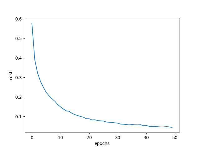
After 50 epochs of training, the accuracy on training set is: 98.94 %. Accuracy on test set is: 98.55 %.
Lastly, the training process cost me 2936 seconds, about 50 minutes. This is notably slower than the multi-layer neural network as shown in a previous post.
Summary
In this post we assembled the building blocks of a convolution neural
network and created from scratch 2 numpy implementations. The unified
interface design permits flexible CNN architectures, and a 6-layer CNN
is created by mixing 2 convolution layers, 1 max-pooling layer, 1
flatten layer and 2 fully connected layers. Using this CNN, we
classified MNIST hand-written digits and managed to achieve comparable
level of accuracy as the multi-layer neural network
shown previously.


