In a previous post I introduced CDAT as a Python package for the manipulation of netCDF data, and made some comparisons with netcdf4. In my own opinion, implementations like CDAT, Iris and Xarray stick to the netCDF philosophy better than netcdf4, in that they permit meta-data preserving operations. Compared with Xarray, CDAT‘s array manipulation API is closer to native numpy.

In this post, and a number of posts to follow, I’d like to share some experiences using CDAT. I’ll start from installation, some basic file reading and saving, then move onto array manipulation, meta-data maintenance, etc., before covering some more advanced topics. So stay tuned if you are interested in learning this power tool.

Platform

CDAT is supported in Linux or MacOS. If you can setup a WSL ("Windows Subsystem for Linux"), it can be used in Windows 10 as well (although technically it is still running inside Linux). Of cause you can create a Linux virtual machine inside Windows to achieve the similar effects but at a greater cost of system resources. The CDAT team provides some very detailed instructions on how to setup a WSL for CDAT installation.

In this post I will only show the installation in Linux. The process in MacOS is the same. Aside from the setting-up of WSL or a virtual machine, the subsequent installation in Windows is also the same.

Install CDAT in Linux

Installation of CDAT has become way easier than before with the help of conda. When I first learned CDAT about 8 years ago, I had to compile all the dependencies myself, then configure and compile CDAT from source code.

This wiki page gives full instructions on the installation of Anaconda or Miniconda (a lighter-weight version of the former), and the installation of CDAT via conda. I’ll only show the steps to install the "lite" version of CDAT, which contains only the core data array manipulation modules, leaving out the virtualization-related modules. For plot creation we will be using the matplotlib+Cartopy combination.

Step 1: Install Anaconda

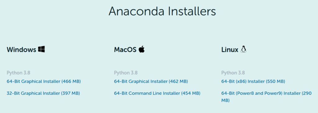
Go to the download page of Anaconda, download the installer for Linux (labeled as "64-Bit (x86) Installer" in the screenshot below):

Once finished, you will get a file with a name like Anaconda3-2020.02-Linux-x86_64.sh. Navigate to the folder storing this file in a terminal, then run:

bash ./Anaconda3-2020.02-Linux-x86_64.sh

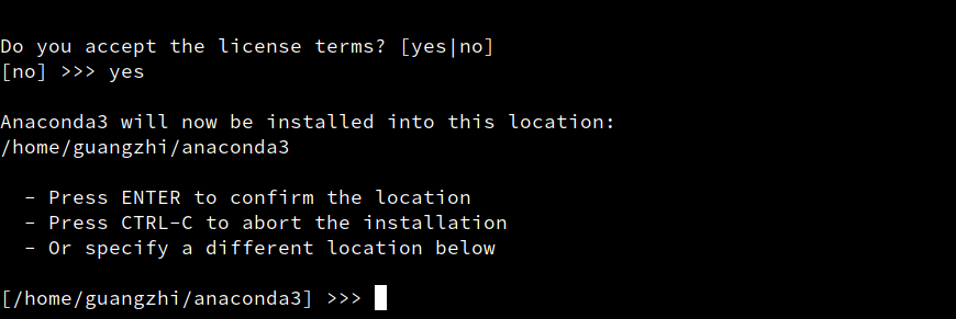
This will launch the command-line installer. Just follow the instructions given within. Specifically, when asked about an installation location (see Figure 2 below), choose the default (which is the anaconda3 folder in your HOME folder).

After seeing installation finished being printed out to the terminal, it will prompt you to decide

Do you wish the installer to initialize Anaconda3
by running conda init? [yes|no]

Type yes and ENTER.

Remember to close the terminal window and open a new one to finalize the anaconda installation.

Step 2: Create a new conda environment

A Python environment is an isolated virtual space in the system. Inside the environment one can install Python packages that are isolated from those in other environments, so that different versions of the same packages, or even different versions of Python, can co-exist in the same system. This way, one can create different environments, with different packages, for different workflows or tasks.

It is advised to always build up your Python working environment from an empty one, so that the chance of package conflicts can be minimized, and if anything goes wrong, it is easier to destroy the compromised environment and start afresh.

To create a new environment (or env for short) for CDAT installation:

conda create -n cdat python=3

The -n cdat part specifies the name of the environment, you can choose a different name if you like. In the remaining part of the command you can specify what packages to install upon env creation. In this case we only specify the Python version to be 3. You can also be more specific about the version by using, for instance, python=3.7.

When finished, activate the environment:

conda activate cdat

[As a side note, in Windows, you will be using activate cdat instead to activate an env. Since I’m assuming you are doing this in WSL or a Linux virtual machine, the activation command would be conda activate.]

After that the shell prompt will be prepended with the env name, like:

(cdat):$

Another side note: if you use a specific environment frequently, it may be worth adding the activation command to the .bashrc file, so that the env is activated in every new terminal session.

Step 3: Install packages

Make sure you are already in the newly created cdat environment. Then we’ll install the 2 core module of CDAT – cdms2 and cdutil, plus a few extra numerical (scipy and pandas) and plotting packages (matplotlib and cartopy) that one is almost certainly gonna use sooner or later. You can add your own choices to the list, or install them separately when in need.

The installation command is:

conda install -c conda-forge scipy pandas matplotlib cartopy cdms2 cdutil

Then validate the installation:

python -c "import cdms2, MV2, cdtime"

If nothing prints out, installation is done.