
The problem
When examining the relationships between multiple time series or sequences, it is often plausible to plot them in a single graph so that their variations can be seen simultaneously. However, when the time series/sequences have very different scales, for instance, one changes from 1 to 10 while the other varies on an order of thousands, it can be difficult to visualize both of them on a single y-axis. In such cases, a common solution is to plot the 2nd sequence on a separate y-axis on the right hand side of the graph, and let the 2 y-axes share the same x-axis. This can be extended to include a 3rd, or more y-axes if needed.
In matplotlib, a secondary y-axis sharing the same x-axis with
another one is called a twin axis, and can be created using: twinax = ax.twinx(). Then, this new axis can be used to plot a different
sequence, just like in a normal line plot:
twinax.plot(x, y2, label='2nd y')
One issue arising from this approach is that these 2 y-axes have independent axis ticks, which in general won’t align up. See Figure 1 for an example:
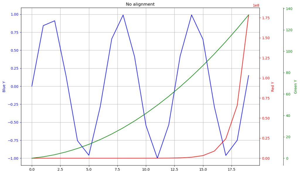
In this example there are 3 different y sequences, 1 on the left and 2
on the right. The curves are plotted onto the y-axes of their
corresponding color. Note that they all have very different scales
(the red one varies from 0 to 10^8, see the scaling factor at the top
of the plot). The grid lines are turned on, to highlight the
misalignment of the y-axes ticks.
The solution
You may find some relevant solutions on the internet, for instance, in this Stackoverflow post. However, most of them only allow you to align up a pair of axes, or only a pair of chosen ticks in a pair of axes (e.g. align up 0 on the left y-axis with 100 on the right). These don’t solve the problem satisfactorily enough, in my option. So I went on to work out my own.
Here is the figure showing the result of my solution:
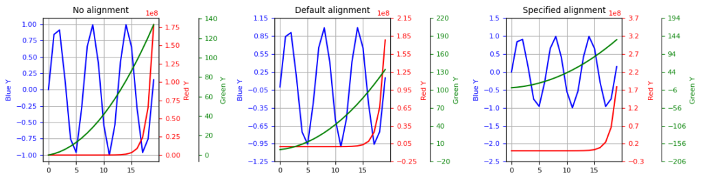
- Left column: original plot without tick alignment.
- Mid column: align ticks using the minimum value in each y sequence.
- Right column: specify some values to align up with:
0for the blue y-axis,2.2 * 1e8for the red and44for the green. These are all chosen arbitrarily.
The function to achieve this:
def alignYaxes(axes, align_values=None):
    '''Align the ticks of multiple y axes

    Args:
        axes (list): list of axes objects whose yaxis ticks are to be aligned.
    Keyword Args:
        align_values (None or list/tuple): if not None, should be a list/tuple
            of floats with same length as <axes>. Values in <align_values>
            define where the corresponding axes should be aligned up. E.g.
            [0, 100, -22.5] means the 0 in axes[0], 100 in axes[1] and -22.5
            in axes[2] would be aligned up. If None, align (approximately)
            the lowest ticks in all axes.
    Returns:
        new_ticks (list): a list of new ticks for each axis in <axes>.

        A new sets of ticks are computed for each axis in <axes> but with equal
        length.
    '''
    from matplotlib.pyplot import MaxNLocator

    nax=len(axes)
    ticks=[aii.get_yticks() for aii in axes]
    if align_values is None:
        aligns=[ticks[ii][0] for ii in range(nax)]
    else:
        if len(align_values) != nax:
            raise Exception("Length of <axes> doesn't equal that of <align_values>.")
        aligns=align_values

    bounds=[aii.get_ylim() for aii in axes]

    # align at some points
    ticks_align=[ticks[ii]-aligns[ii] for ii in range(nax)]

    # scale the range to 1-100
    ranges=[tii[-1]-tii[0] for tii in ticks]
    lgs=[-np.log10(rii)+2. for rii in ranges]
    igs=[np.floor(ii) for ii in lgs]
    log_ticks=[ticks_align[ii]*(10.**igs[ii]) for ii in range(nax)]

    # put all axes ticks into a single array, then compute new ticks for all
    comb_ticks=np.concatenate(log_ticks)
    comb_ticks.sort()
    locator=MaxNLocator(nbins='auto', steps=[1, 2, 2.5, 3, 4, 5, 8, 10])
    new_ticks=locator.tick_values(comb_ticks[0], comb_ticks[-1])
    new_ticks=[new_ticks/10.**igs[ii] for ii in range(nax)]
    new_ticks=[new_ticks[ii]+aligns[ii] for ii in range(nax)]

    # find the lower bound
    idx_l=0
    for i in range(len(new_ticks[0])):
        if any([new_ticks[jj][i] > bounds[jj][0] for jj in range(nax)]):
            idx_l=i-1
            break

    # find the upper bound
    idx_r=0
    for i in range(len(new_ticks[0])):
        if all([new_ticks[jj][i] > bounds[jj][1] for jj in range(nax)]):
            idx_r=i
            break

    # trim tick lists by bounds
    new_ticks=[tii[idx_l:idx_r+1] for tii in new_ticks]

    # set ticks for each axis
    for axii, tii in zip(axes, new_ticks):
        axii.set_yticks(tii)

    return new_ticks
Some more explanations
The alignYaxes() function first takes the tick values generated by
matplotlib, and scales them down to the range of 1-100. With a unified
variation range, we can merge these scaled tick values into a single
sequence, and let matplotlib create a new set of ticks for us, as if
they all belong to the same y- array. This new set of ticks is created
using the MaxNLocator:
comb_ticks=np.concatenate(log_ticks)
comb_ticks.sort()
locator=MaxNLocator(nbins='auto', steps=[1, 2, 2.5, 3, 4, 5, 8, 10])
new_ticks=locator.tick_values(comb_ticks[0], comb_ticks[-1])
Then the new tick values are scaled back, using the scaling factor of each y-axis, to their original scales. Thus, we obtain the equal number of ticks for each sequence, and they all have nice looking figures.
If some specific alignment values are provided, a shift is performed before scaling, and another shift afterwards to restore the offset. This creates the right column plot in Figure 2.
Complete code
Complete script to generate Figure 2:
import matplotlib.pyplot as plt
import numpy as np

def make_patch_spines_invisible(ax):
    '''Used for creating a 2nd twin-x axis on the right/left

    E.g.
        fig, ax=plt.subplots()
        ax.plot(x, y)
        tax1=ax.twinx()
        tax1.plot(x, y1)
        tax2=ax.twinx()
        tax2.spines['right'].set_position(('axes',1.09))
        make_patch_spines_invisible(tax2)
        tax2.spines['right'].set_visible(True)
        tax2.plot(x, y2)
    '''

    ax.set_frame_on(True)
    ax.patch.set_visible(False)
    for sp in ax.spines.values():
        sp.set_visible(False)

def alignYaxes(axes, align_values=None):
    '''Align the ticks of multiple y axes

    Args:
        axes (list): list of axes objects whose yaxis ticks are to be aligned.
    Keyword Args:
        align_values (None or list/tuple): if not None, should be a list/tuple
            of floats with same length as <axes>. Values in <align_values>
            define where the corresponding axes should be aligned up. E.g.
            [0, 100, -22.5] means the 0 in axes[0], 100 in axes[1] and -22.5
            in axes[2] would be aligned up. If None, align (approximately)
            the lowest ticks in all axes.
    Returns:
        new_ticks (list): a list of new ticks for each axis in <axes>.

        A new sets of ticks are computed for each axis in <axes> but with equal
        length.
    '''
    from matplotlib.pyplot import MaxNLocator

    nax=len(axes)
    ticks=[aii.get_yticks() for aii in axes]
    if align_values is None:
        aligns=[ticks[ii][0] for ii in range(nax)]
    else:
        if len(align_values) != nax:
            raise Exception("Length of <axes> doesn't equal that of <align_values>.")
        aligns=align_values

    bounds=[aii.get_ylim() for aii in axes]

    # align at some points
    ticks_align=[ticks[ii]-aligns[ii] for ii in range(nax)]

    # scale the range to 1-100
    ranges=[tii[-1]-tii[0] for tii in ticks]
    lgs=[-np.log10(rii)+2. for rii in ranges]
    igs=[np.floor(ii) for ii in lgs]
    log_ticks=[ticks_align[ii]*(10.**igs[ii]) for ii in range(nax)]

    # put all axes ticks into a single array, then compute new ticks for all
    comb_ticks=np.concatenate(log_ticks)
    comb_ticks.sort()
    locator=MaxNLocator(nbins='auto', steps=[1, 2, 2.5, 3, 4, 5, 8, 10])
    new_ticks=locator.tick_values(comb_ticks[0], comb_ticks[-1])
    new_ticks=[new_ticks/10.**igs[ii] for ii in range(nax)]
    new_ticks=[new_ticks[ii]+aligns[ii] for ii in range(nax)]

    # find the lower bound
    idx_l=0
    for i in range(len(new_ticks[0])):
        if any([new_ticks[jj][i] > bounds[jj][0] for jj in range(nax)]):
            idx_l=i-1
            break

    # find the upper bound
    idx_r=0
    for i in range(len(new_ticks[0])):
        if all([new_ticks[jj][i] > bounds[jj][1] for jj in range(nax)]):
            idx_r=i
            break

    # trim tick lists by bounds
    new_ticks=[tii[idx_l:idx_r+1] for tii in new_ticks]

    # set ticks for each axis
    for axii, tii in zip(axes, new_ticks):
        axii.set_yticks(tii)

    return new_ticks

def plotLines(x, y1, y2, y3, ax):

    ax.plot(x, y1, 'b-')
    ax.set_ylabel('Blue Y', color='b')
    ax.tick_params('y',colors='b')

    tax1=ax.twinx()
    tax1.plot(x, y2, 'r-')
    tax1.set_ylabel('Red Y', color='r')
    tax1.tick_params('y',colors='r')

    tax2=ax.twinx()
    tax2.spines['right'].set_position(('axes',1.34))
    make_patch_spines_invisible(tax2)
    tax2.spines['right'].set_visible(True)
    tax2.plot(x, y3, 'g-')
    tax2.set_ylabel('Green Y', color='g')
    tax2.tick_params('y',colors='g')

    ax.grid(True, axis='both')

    return ax, tax1, tax2

#-------------Main---------------------------------
if __name__=='__main__':

    # craft some data to plot
    plt.rcParams.update({'font.size': 8})

    x=np.arange(20)
    y1=np.sin(x)
    y2=x/1000+np.exp(x)
    y3=x+x**2/3.14

    figure=plt.figure(figsize=(12,3),dpi=100)

    ax1=figure.add_subplot(1, 3, 1)
    axes1=plotLines(x, y1, y2, y3, ax1)
    ax1.set_title('No alignment')

    ax2=figure.add_subplot(1, 3, 2)
    axes2=plotLines(x, y1, y2, y3, ax2)
    alignYaxes(axes2)
    ax2.set_title('Default alignment')

    ax3=figure.add_subplot(1, 3, 3)
    axes3=plotLines(x, y1, y2, y3, ax3)
    alignYaxes(axes3, [0, 2.2*1e8, 44])
    ax3.set_title('Specified alignment')

    figure.subplots_adjust(wspace=1.)
    figure.show()


Hey,
Thanks a lot for the code, super helpful!
Just a note that in some cases, I’ve found that using igs=[np.round(ii) for ii in lgs] instead of igs=[np.floor(ii) for ii in lgs] gives better results. For instance, in one case I had ticks ranging from 0 to 9e-2 on the left axis and from -.2 to 1.2 on the right axis. Using np.floor() would squish the right axis, whereas np.round() extends the left one, and the result looks better in my opinion.
Anyway, thanks very much again!
Cheers,
Pierre
Thanks Pierre for the comment.
I didn’t give it too much thought when using the `floor` function. Will change mine to `round`.