The Ramer-Douglas-Peucker (RDP) algorithm
The Ramer-Douglas-Peucker (RDP) algorithm is a curve simplification method. The idea of RDP is that the interior points along a non-closed curve are recursively examined and removed, if the removal of a point does not introduce an error in the curve placement beyond a given upper bound. Figure 1 below gives an example of this process.
[latexpage]
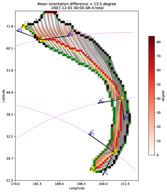
A curve is defined as a sorted sequence \(P1 – P5\) . In the first iteration, it finds the point (\(P2\)) that is furthest from the line segment linking the 2 end points (\(P1\), \(P5\)). This distance \(L\) is the length of \(P_2 P_c\) . \(P2\) is removed if \(L\) is smaller than a user-defined error limit \(\epsilon\), or retained otherwise. Then the process descends into the next recursion using \(P2\) and \(P5\) as end points. The result of this process is that a perfectly straight sequence will be reduced to its two end points, and a complex curve is reduced to a simpler one consisting of a subset of the original points. Therefore the number of segments is not pre-defined but determined by the allowable error, in other words, an axis point is only retained when necessary.
P1 − P5. The point that is furthest from the line segment P1P5 is P2 , and the distance L is the length of P2Pc. The green dashed line denotes the line segment examined in the next recursive call of the algorithm.Below is a Python implementation of the RDP algorithm, translated from the pseudo-code in this wikipedia page.
from math import sqrt

def distance(a, b):
    '''Euclidean distance between 2 points
    Args:
        a (tuple): (x, y) coordinates of point A.
        b (tuple): (x, y) coordinates of point B.
    Returns:
        result (float): Euclidean distance between 2 points
    '''
    return  sqrt((a[0] - b[0]) ** 2 + (a[1] - b[1]) ** 2)

def point_line_distance(point, start, end):
    '''Eucliean distance between a point and a line
    Args:
        point (tuple): (x, y) coordinates of a point.
        start (tuple): (x, y) coordinates of the starting point of a line.
        end (tuple): (x, y) coordinates of the end point of a line.
    Returns:
        result (float): shortest distance from point to line.
    '''
    if (start == end):
        return distance(point, start)
    else:
        n = abs((end[0]-start[0])*(start[1]-point[1])-\
                (start[0]-point[0])*(end[1]-start[1]))
        d = sqrt((end[0]-start[0])**2+(end[1]-start[1])**2)

        return n / d

def rdp(points, epsilon):
    '''Reduces a series of points to a simplified version that loses detail, but
    maintains the general shape of the series.

    Args:
        points (list): a list of (x, y) coordinates forming a simple curve.
        epsilon (float): error threshold.
    Returns:
        results (list): a list of (x, y) coordinates of simplified curve.
    '''
    dmax = 0.0
    index =
    for i in range(1, len(points) - 1):
        d = point_line_distance(points[i], points[0], points[-1])
        if d > dmax:
            index = i
            dmax = d
    if dmax >= epsilon:
        results = rdp(points[:index+1], epsilon)[:-1] + rdp(points[index:], epsilon)
    else:
        results=[points[0],points[-1]]

    return results
Spherical geometry
The above RDP algorithm is using geometries in the Cartesian coordinates, which can be used for latitude/longitude coordinates if the scale is not too large (perhaps within a couple of kilometers). However, when the scale goes above a few degrees of latitude/longitude, the effects from the curvature of the Earth surface would start to kick in, and one needs to replace the geometries with a spherical one.
There are two parts of the Cartesian geometry that need to be replaced:
- distance between 2 given points.
- distance between a point and a line.
The great circle distance: shortest distance on the sphere surface
The shortest distance on a unit sphere is defined as the great circle distance, which is the length of the arc connecting 2 points on the sphere, where the arc is on a circle which is obtained by cutting the sphere with a plane that goes through the origin.
The great circle distance is computed as:
[latexpage]
\[
\Delta \sigma = \arctan \frac{\sqrt{(\cos \phi_2 \sin \Delta \lambda)^2 + (\cos \phi_1 \sin \phi_2 – \sin \phi_1 \cos \phi_2 \cos \Delta \lambda)^2}}{ \sin \phi_1 \sin \phi_2 + \cos \phi_1 \cos \phi_2 cos \Delta \lambda}
\]
where \(\phi_1\), \(\lambda_1\) are the start point latitude and longitude, respectively. And \(\phi_2\) and \(\lambda_2\) are the end point coordinates. \(\Delta \lambda\) is the difference in longitude.
Note that this is the distance on a unit sphere, for spheres with non-unit radius, one needs to multiple \(\Delta \sigma\) with the radius \(R\).
Below is the Python code for the great circle distance computation:
def greatCircle(lat1,lon1,lat2,lon2,r=None,verbose=False):
    '''Compute the great circle distance on a sphere

    <lat1>, <lat2>: scalar float or nd-array, latitudes in degree for
                    location 1 and 2.
    <lon1>, <lon2>: scalar float or nd-array, longitudes in degree for
                    location 1 and 2.

    <r>: scalar float, spherical radius.

    Return <arc>: great circle distance on sphere.
    '''

    from numpy import sin, cos

    if r is None:
        r=6371000. #m

    d2r=lambda x:x*np.pi/180
    lat1,lon1,lat2,lon2=map(d2r,[lat1,lon1,lat2,lon2])
    dlon=abs(lon1-lon2)

    numerator=(cos(lat2)*sin(dlon))**2 + \
            (cos(lat1)*sin(lat2) - sin(lat1)*cos(lat2)*cos(dlon))**2
    numerator=np.sqrt(numerator)
    denominator=sin(lat1)*sin(lat2)+cos(lat1)*cos(lat2)*cos(dlon)

    dsigma=np.arctan2(numerator,denominator)
    arc=r*dsigma

    return arc
Cross-track distance: the shortest distance between a point and a "line" on the sphere surface
[latexpage]
On the sphere surface, a “straight line” is replaced with the great circle arc linking 2 points. Therefore, the distance between a point and the arc is also measured using great circle distance. When the start (\(P1\)) and end (\(P2\)) points of the arc overlap, the problem regresses back to problem 1, i.e. great circle distance between 2 points (between \(P1/P2\) and \(P3\)). In the general case when the start and end points are separate, the spherical equivalent to the distance \(P_2P_c\) is called cross-track distance, which can be computed using the formula given in http://www.movable-type.co.uk/scripts/latlong.html:
\[
d_{xt} = \arcsin( \sin( \delta_{13}) \sin(\theta_{13} – \theta_{12})) R
\]
where:
- \(\delta_{13}\) is (angular) distance from start point (P1) to third point (P3).
- \(\theta_{13}\) is (initial) bearing from start point (P1) to third point (P3).
- \(\theta_{12}\) is (initial) bearing from start point (P1) to end point (P2).
- \(R\) is the radius of the sphere.
The initial bearing (aka forward azimuth) is the angle between North and the direction facing from a start point to the end point. In general, the heading direction changes as one travels along a great circle, and the initial bearing is the heading direction at the starting point. The convention is that bearing starts from 0 degree at the North direction, increases clock-wise to 180 degree to the South direction, and back to North at 360 degree.
Bearing is computed using the formula from the above reference:
[latexpage]
\[
\theta = arctan2( \sin \Delta \lambda \cos \phi_2, \cos \phi_1 \sin
\phi_2 – \sin \phi_1 \cos \phi_2 \cos \Delta \lambda)
\]
where \(\phi_1\), \(\lambda_1\) are the start point latitude and longitude, respectively. And \(\phi_2\) and \(\lambda_2\) are the end point coordinates. \(\Delta \lambda\) is the difference in longitude.
The Python implementation of the computation of cross-track distance is given below:
def getBearing(lat1,lon1,lat2,lon2):
    '''Compute bearing from point 1 to point2

    Args:
        lat1,lat2 (float or ndarray): scalar float or nd-array, latitudes in
            degree for location 1 and 2.
        lon1,lon2 (float or ndarray): scalar float or nd-array, longitudes in
            degree for location 1 and 2.
    Returns:
        theta (float or ndarray): (forward) bearing in degree.

    NOTE that the bearing from P1 to P2 is in general not the same as that
    from P2 to P1.
    '''
    from numpy import sin, cos

    d2r=lambda x:x*np.pi/180
    lat1,lon1,lat2,lon2=map(d2r,[lat1,lon1,lat2,lon2])
    dlon=lon2-lon1
    theta=np.arctan2(sin(dlon)*cos(lat2),
            cos(lat1)*sin(lat2)-sin(lat1)*cos(lat2)*cos(dlon))
    theta=theta/np.pi*180
    theta=(theta+360)%360

    return theta


def getCrossTrackDistance(lat1,lon1,lat2,lon2,lat3,lon3,r=None):
    '''Compute cross-track distance

    Args:
        lat1, lon1 (float): scalar float or nd-array, latitudes and longitudes in
                        degree, start point of the great circle.
        lat2, lon2 (float): scalar float or nd-array, latitudes and longitudes in
                        degree, end point of the great circle.
        lat3, lon3 (float): scalar float or nd-array, latitudes and longitudes in
                        degree, a point away from the great circle.
    Returns:
        dxt (float): great cicle distance between point P3 to the closest point
                  on great circle that connects P1 and P2.

                  NOTE that the sign of dxt tells which side of the 3rd point
                  P3 is on.

    See also getCrossTrackPoint(), getAlongTrackDistance().
    '''
    from numpy import sin

    if r is None:
        r=6371000.  #m

    # get angular distance between P1 and P3
    delta13=greatCircle(lat1,lon1,lat3,lon3,r=1.)
    # bearing between P1, P3
    theta13=getBearing(lat1,lon1,lat3,lon3)*np.pi/180
    # bearing between P1, P2
    theta12=getBearing(lat1,lon1,lat2,lon2)*np.pi/180

    dtheta=np.arcsin(sin(delta13)*sin(theta13-theta12))
    dxt=r*dtheta

    return dxt
Python code for the spherical version of RDP
With these 2 spherical geometry components solved, the spherical RDP can be implemented in Python using:
def distanceGC(a,b):
    '''Great circle distance

    Args:
        a (tuple): (lat, lon) coordinates of point A.
        b (tuple): (lat, lon) coordinates of point B.
    Returns:
        result (float): great circle distance from A to B, on unit sphere.
    '''
    return greatCircle(a[0],a[1],b[0],b[1],r=1)

def point_line_distanceGC(point,start,end):
    '''Shortest distance between a point and a great circle curve on unit sphere

    Args:
        point (tuple): (lon, lat) coordinates of a point on unit sphere.
        start (tuple): (lon, lat) coordinates of the starting point of a curve
            on unit sphere.
        end (tuple): (lon, lat) coordinates of the end point of a curve
            on unit sphere.
    Returns:
        result (float): shortest distance from point to line.
    '''
    if (start == end):
        return distanceGC(point, start)/np.pi*180.
    else:
        dxt=getCrossTrackDistance(start[0],start[1],
                end[0],end[1],
                point[0],point[1],
                r=1)

        dxt=abs(dxt/np.pi*180)
        return dxt

def rdpGC(points, epsilon):
    '''Geodesic version of rdp.

    Args:
        points (list): list of (lon, lat) coordinates on unit sphere.
        epsilon (float): error threshold.
    Returns:
        results (list): a list of (lon, lat) coordinates of simplified curve.
    '''

    dmax = 0.0
    index = 0
    for i in range(1, len(points) - 1):
        d = point_line_distanceGC(points[i], points[0], points[-1])
        if d > dmax:
            index = i
            dmax = d
    if dmax >= epsilon:
        results = rdpGC(points[:index+1], epsilon)[:-1] + rdpGC(points[index:], epsilon)
    else:
        results=[points[0],points[-1]]

    return results
An example
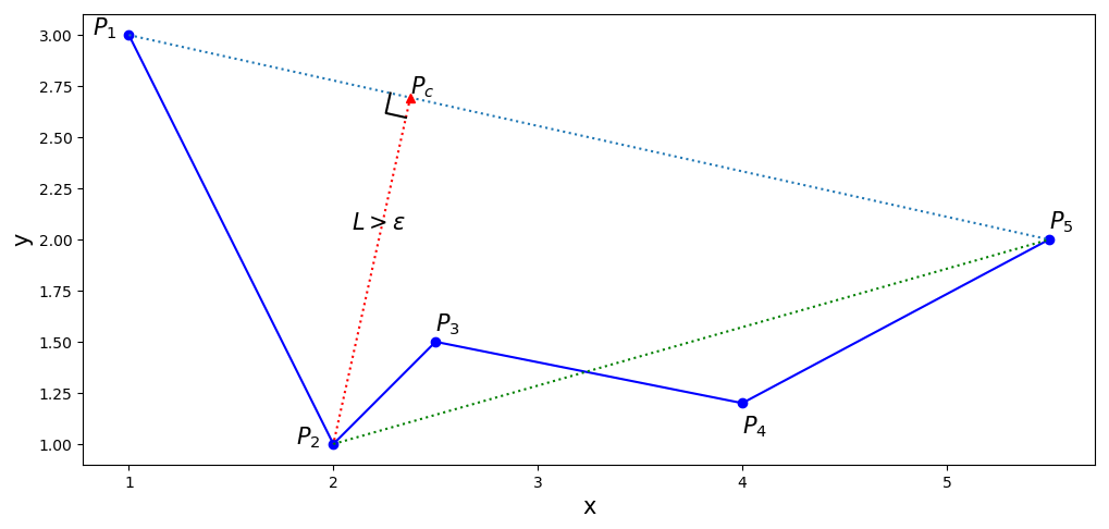
Figure 2 gives an example of the spherical RDP algorithm. The plot shows one atmospheric river (AR) viewed from top-down. AR is a phenomenon observed in the mid-lower troposphere where a large plume of water vapor is being transported by some strong horizontal winds, such that when viewed from satellite imagery or gridded atmospheric data, they appear as elongated vapor filaments, somehow like terrestrial rivers.
We can omit all the other elements of the plot and only focus on the red dotted line. That is the axis of this atmospheric river. The spacing of the red dots is about 80 km apart, so you can get a general idea about the length of this river. There are too many red dots in the axis, and I wanted to cut the river into a fewer number of segments such that within each segment, the orientation of the axis is more or less the same. In other words, this is a curve simplification task, done using latitude/longitude coordinates. That’s why we need a spherical version the of the RDP algorithm.
The result of the RDP simplification is drawn using yellow squares and lines. The orientation error to the RDP algorithm is 2 degrees of latitude/longitude. Therefore, within each of the segments, e.g. $P0P1$ or $P1P2$, the red axis curve never deviates from the simplified yellow curve by more than 2 degrees.