The goal
In a previous post we implemented 2D and 3D convolutions using
numpy. That is one major building block of a convolution neural
network (CNN). However, to train a new CNN one also needs to
implement error back-propagation, which will be the topic of this post.
Recap on convolution layer and notations
Before going into the back-propagation, it is necessary to understand what the forward computation is doing. Below is a brief recapture on the forward pass and some notations.
For a convolution layer which is the lth layer in the CNN, we denote:
- \(f^{(l)}\): height and width of the convolution kernel/filter.
- \(n^{(l)}_c\): number of filters in the convolution layer.
- \(n^{(l-1)}_H \times n^{(l-1)}_W \times n^{(l-1)}_c\): size of the input to the convolution layer, i.e. activation of layer \(l-1\), as the product of height (\(n^{(l-1)}_H\)), width (\(n^{(l-1)}_W\)) and number of channels (\(n^{(l-1)}_c\)).
- \(n^{(l)}_H \times n^{(l)}_W \times n^{(l)}_c\): size of the output of the convolution layer.
- \(w^{(l,k)}\): the kth convolution kernel/filter of layer \(l\): \(w^{(l,k)} \in \mathbb{R}^{f^{(l)} \times f^{(l)}}\).
- \(z^{(l,k)}\): convolution result from the kth filter: \(z^{(l,k)} \in \mathbb{R}^{n^{(l)}_H \times n^{(l)}_W}\).
- \(z^{(l)}\): stacked convolution results from all filters: \(z^{(l)} \in \mathbb{R}^{n^{(l)}_H \times n^{(l)}_W \times n^{(l)}_c}\).
- \(b^{(l, k)}\): bias term for the kth filter in the layer: \(b^{(l,k)} \in \mathbb{R}\).
- \(b^{(l)}\): bias term for all the filters in the layer: \(b^{(l)} \in \mathbb{R}^{n^{(l)}_c}\).
- \(a^{(l,k)}\): result of the activation function for the kth filter in the layer: \(a^{(l, k)} \in \mathbb{R}^{n^{(l)}_H \times n^{(l)}_W}\).
- \(a^{(l)}\): result of the activation function for all the filters in the layer: \(a^{(l)} \in \mathbb{R}^{n^{(l)}_H \times n^{(l)}_W \times n^{(l)}_c}\).
Take for instance the convolution layer shown in Figure 1 below. The input to the layer is denoted \(a^{(l-1)}\), which is also the activation of layer \(l-1\). In the case shown in Figure xxx \(a^{(l-1)}\) is a 2D array, but recall that in general \(a^{(l-1)}\) is a 3D data volume.
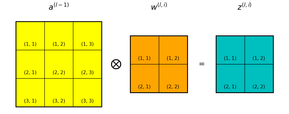
\(w^{(l,k)}\) is the kth convolution kernel/filter in the convolution layer.
The convolution process is given as:
\[
z^{(l,k)} = a^{(l-1)} \otimes w^{(l,k)}
\]
where \(\otimes\) is the convolution operator.
Then a bias term \(b^{(l,k)} \in \mathbb{R}\) is added to the convolution result:
\[
z^{(l,k)} = a^{(l-1)} \otimes w^{(l,k)} + b^{(l,k)}
\]
Then, the convolution result is passed to an activation function \(g()\):
\[
a^{(l,k)} = g(z^{(l,k)}) = g(a^{(l-1)} \otimes w^{(l,k)} + b^{(l,k)})
\]
After repeating the same process for all of the \(n^{(l)}_c\) filters in the layer and stacking up the results, the output of the convolution layer is \(a^{(l)} \in \mathbb{R}^{n^{(l)}_H \times n^{(l)}_W \times n^{(l)}_c}\).
Finally, we denote the loss function of the CNN as \(J\), and the error term of layer \(l\) as:
\[
\frac{\partial J}{\partial z^{(l)}} \equiv \delta^{(l)}
\]
Back-propagation in a 2D convolution layer
Computation of weight gradients
Take again the above example in Figure 1. To simplify the derivations
I’m omitting the filter index k and assuming that there is only a single
filter in the convolution layer.
Let’s write out the convolution process of \(z^{(l)} = a^{(l-1)} \otimes w^{(l)}\):
\[
\left\{\begin{matrix}
z_{1,1} = & a_{1,1} w_{1,1} + a_{1,2} w_{1,2} + a_{2,1} w_{2,1} + a_{2,2} w_{2,2} \\
z_{1,2} = & a_{1,2} w_{1,1} + a_{1,3} w_{1,2} + a_{2,2} w_{2,1} + a_{2,3} w_{2,2} \\
z_{2,1} = & a_{2,1} w_{1,1} + a_{2,2} w_{1,2} + a_{3,1} w_{2,1} + a_{3,2} w_{2,2} \\
z_{2,2} = & a_{2,2} w_{1,1} + a_{2,3} w_{1,2} + a_{3,2} w_{2,1} + a_{3,3} w_{2,2} \\
\end{matrix}\right.
\] [Eq. 1]
Note that the z terms are for layer l and a terms are from
layer l-1, I’m omitting the superscripts for brevity. The subscript
indices denote the row,column positions of the pixels, as shown in
Figure 1.
To update the weights we need to compute their gradients \(\frac{\partial J}{\partial w^{(l)}_{i,j}}\), where \(l\) denotes layer \(l\), \(i\) and \(j\) denote the row/column indices of a number in the filter.
By applying the chain rule on the 1st element of the weight matrix \(w_{1,1}\) and using Equation 1:
\[
\frac{\partial J}{\partial w_{1,1}} = \frac{\partial J}{\partial z_{1,1}} \frac{\partial z_{1,1}}{\partial w_{1,1}} +
\frac{\partial J}{\partial z_{1,2}} \frac{\partial z_{1,2}}{\partial w_{1,1}} +
\frac{\partial J}{\partial z_{2,1}} \frac{\partial z_{2,1}}{\partial w_{1,1}} +
\frac{\partial J}{\partial z_{2,2}} \frac{\partial z_{2,2}}{\partial
w_{1,1}}
\] [Eq 2]
Note I’m omitting the superscript \(^{(l)}\) for all the \(w\) and \(z\) terms in the above equation.
Notice that \(\frac{\partial J}{\partial z_{1,1}}\) is \(\delta_{1,1}\) by definition, and \(\frac{\partial z_{1,1}}{\partial w_{1,1}} = a_{1,1}\) from Equation 1. We can similarly replace all other terms in Equation 2 to get:
\[
\frac{\partial J}{\partial w_{1,1}} = \delta_{1,1} a_{1,1} +
\delta_{1,2} a_{1,2} +
\delta_{2,1} a_{2,1} +
\delta_{2,2} a_{2,2}
\]
That gives the gradient for the first element in the weight matrix. Repeating the same process we get the gradients for all the elements in weight \(w^{(l)}\):
\[
\left\{\begin{matrix}
\frac{\partial J}{\partial w^{(l)}_{1,1}} = & \delta^{(l)}_{1,1} a^{(l-1)}_{1,1} + \delta^{(l)}_{1,2} a^{(l-1)}_{1,2} + \delta^{(l)}_{2,1} a^{(l-1)}_{2,1} + \delta^{(l)}_{2,2} a^{(l-1)}_{2,2} \\
\frac{\partial J}{\partial w^{(l)}_{1,2}} = & \delta^{(l)}_{1,1} a^{(l-1)}_{1,2} + \delta^{(l)}_{1,2} a^{(l-1)}_{1,3} + \delta^{(l)}_{2,1} a^{(l-1)}_{2,2} + \delta^{(l)}_{2,2} a^{(l-1)}_{2,3} \\
\frac{\partial J}{\partial w^{(l)}_{2,1}} = & \delta^{(l)}_{1,1} a^{(l-1)}_{2,1} + \delta^{(l)}_{1,2} a^{(l-1)}_{2,2} + \delta^{(l)}_{2,1} a^{(l-1)}_{3,1} + \delta^{(l)}_{2,2} a^{(l-1)}_{3,2} \\
\frac{\partial J}{\partial w^{(l)}_{2,2}} = & \delta^{(l)}_{1,1} a^{(l-1)}_{2,2} + \delta^{(l)}_{1,2} a^{(l-1)}_{2,3} + \delta^{(l)}_{2,1} a^{(l-1)}_{3,2} + \delta^{(l)}_{2,2} a^{(l-1)}_{3,3} \\
\end{matrix}\right.
\]
I’ve added all superscripts to make it clearer which term is from which layer.
It is a pretty complicated equation set at first look. However, it turns out that it can be expressed more neatly as:
\[
\frac{\partial J}{\partial w^{(l)}} = a^{(l-1)} \otimes \delta^{(l)}
\]
namely, a convolution between the error term of the layer \(\delta^{(l)}\) and the input to the layer \(a^{(l-1)}\).
Compare this with the gradient computation in an ordinary neural network layer, where
\[
\frac{\partial J}{\partial \theta^{(l)}} = \delta^{(l)} \cdot a^{(l-1)^T}
\]
we have a similar structure: gradients of a weight (\(\frac{\partial J}{\partial \theta^{(l)}}\)) in a layer is proportional to its input (\(a^{(l-1)}\)) and the error of the output (\(\delta^{(l)}\)).
From Equation 3, we see that to compute the gradients for the weights in a layer, we need to know the inputs into the layer (\(a^{(l-1)}\)), which we can get by saving a copy during the forward propagation process; and the error term \(\delta^{(l)}\) of the layer. For the latter we need to propagate the error all the way from the last layer in the network backwards. This is derived in the next part.
Computation of error back propagation
We now derive the process of propagating the error backwards across a convolution layer. Using again the schematic in Figure 1, we are looking for an expression of \(\delta^{(l-1)}\), given an in-coming error of \(\delta^{(l)}\).
Recall that the error term is defined as \(\delta^{(l-1)} \equiv \frac{\partial J}{\partial z^{(l-1)}}\).
Using the chain rule, we get:
\[
\delta^{(l-1)} \equiv \frac{\partial J}{\partial z^{(l-1)}} = \frac{\partial J}{\partial a^{(l-1)}} \frac{\partial a^{(l-1)}}{\partial z^{(l-1)}}
\]
Note that \(\frac{\partial a^{(l-1)}}{\partial z^{(l-1)}}\) is the derivative of the activation function on \(z^{(l-1)}\):
\[
\frac{\partial a^{(l-1)}}{\partial z^{(l-1)}} = g'(z^{(l-1)})
\]
therefore, it is useful to also save a copy of \(z^{(l-1)}\) during the forward propagation process, and it is also required to know the derivative of the activation function.
Then we need to work out the \(\frac{\partial J}{\partial a^{(l-1)}}\) term in Equation 4.
Notice that \(a^{(l-1)}\) is the input to the convolution layer. Using the chain rule again on the 1st element of \(a^{(l-1)}\):
\[
\frac{\partial J}{\partial a^{(l-1)}_{1,1}} = \frac{\partial J}{\partial z^{(l)}_{1,1}} \frac{\partial z^{(l)}_{1,1}}{\partial a^{(l-1)}_{1,1}} = \delta^{(l)}_{1,1} w^{(l)}_{1,1}
\]
where \(\frac{\partial J}{\partial z^{(l)}_{1,1}} = \delta^{(l)}_{1,1}\) is from the definition of \(\delta\), and \(\frac{\partial z^{(l)}_{1,1}}{\partial a^{(l-1)}_{1,1}} = w^{(l)}_{1,1}\) is from Equation 1.
Write out all elements in \(\frac{\partial J}{\partial a^{(l-1)}}\), we have:
\[
\left\{\begin{matrix}
\frac{\partial J}{\partial a^{(l-1)}_{1,1}} = & \delta^{(l)}_{1,1} w^{(l)}_{1,1} \\
\frac{\partial J}{\partial a^{(l-1)}_{1,2}} = & \delta^{(l)}_{1,1} w^{(l)}_{1,2} + \delta^{(l)}_{1,2}w^{(l)}_{1,1} \\
\frac{\partial J}{\partial a^{(l-1)}_{1,3}} = & \delta^{(l)}_{1,2} w^{(l)}_{1,2} \\
\frac{\partial J}{\partial a^{(l-1)}_{2,1}} = & \delta^{(l)}_{1,1} w^{(l)}_{2,1} + \delta^{(l)}_{2,1}w^{(l)}_{1,1} \\
\cdots & \cdots \\
\frac{\partial J}{\partial a^{(l-1)}_{3,3}} = & \delta^{(l)}_{2,2} w^{(l)}_{2,2} \\
\end{matrix}\right.
\]
It is another monstrous equation set. Fortunately, it can be expressed more neatly again as a convolution:
\[
\frac{\partial J}{\partial a^{(l-1)}} = \delta^{(l)} \otimes_f Rot_{180}(w^{(l)})
\]
where:
- \(\otimes_f\) denotes a “full mode” convolution. See the Convolution modes section in this post for an illustration. In a nutshell, in a “full mode” convolution we compute a dot product between the convolution kernel and the underlying data subset whenever they have any overlap, and as a result, the result from a “full mode” convolution has a larger size than the input. This is also the case as shown in Figure 1.
- \(Rot_{180}()\) is a function that rotates a matrix by 180 degree, or equivalently, flips the matrix horizontally and vertically. Note that in the case of 3D convolution, this does not flip the channel dimension.
Given Equation 5 and Equation 4, we get the formula for error back propagation across a convolution layer:
\[
\delta^{(l-1)} = \delta^{(l)} \otimes_f Rot_{180}(w^{(l)}) \odot g'(z^{(l-1)})
\]
Again, it is interesting to note a similar structure in the back propagation in an ordinary neural network:
\[
\delta^{(l-1)} = \theta^{(l)^T} \cdot \delta^{(l)} \odot g'(z^{(l-1)})
\]
Back-propagation in a 3D convolution layer
The derivations in the above section have made a few simplifications:
- We assume that the input is a 2D array.
- We assume that there is only 1 filter in the convolution layer.
This section will build on top of the previous section and generalize it to cases when the input is a 3D data volume and the convolution layer has more than 1 filters.
Computation of weight gradients
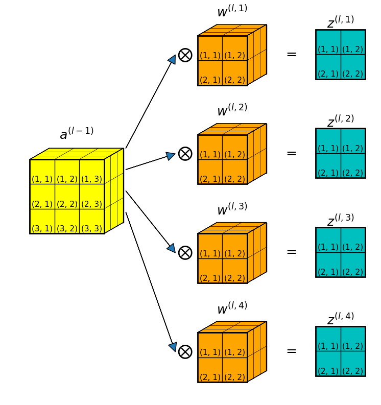
As a concrete example, Figure 2 below shows a convolution layer where:
- the input is a 3D data volume: \(a^{(l-1)} \in \mathbb{R}^{3 \times 3 \times 3}\).
- there are \(4\) filters in the convolution layer, each is a 3D array: \(w^{(l, k)} \in \mathbb{R}^{2 \times 2 \times 3}, \; k=1,2,3,4\).
- for each filter, the convolution produces a 2D slab: \(z^{(l, k)} \in \mathbb{R}^{2 \times 2}, \; k=1,2,3,4\).
- After stacking up all 4 convolution results, the total convolution result is \(z^{(l)} \in \mathbb{R}^{2 \times 2 \times 4}\).
Equation 3 in the above section shows that to get the gradients of filter weights in a 2D convolution with a single filter, we do a convolution between the input (\(a^{(l-1)}\)) and the error (\(\delta^{(l)}\)).
In the case of 3D convolution, it is noticed that there exists a branching-off of the “data flow”: each filter \(w^{(l,k)}\) produces a separate convolution result that is independent to all other filters. Consequently, the weight gradients are computed independently for each filter, using the shared input \(a^{(l-1)}\) and the corresponding error term \(\delta^{(l,k)}\):
\[
\frac{\partial J}{\partial w^{(l, k)}} = a^{(l-1)} \otimes
\delta^{(l,k)}, \; k=1,2,3,4
\]
Note that the shape of \(a^{(l-1)}\) is \(3 \times 3 \times 3\), that of \(\delta^{(l,k)}\) is \(2 \times 2 \times 1\). Therefore the convolution is done 3 times, each for a different channel. This way, we recover the correct shape of the filter: \(w^{(l, k)} \in \mathbb{R}^{2 \times 2 \times 3}\).
Computation of error back propagation
Previously, we have shown in Equation 6 that in a 2D convolution layer with a single filter, the back propagated error across a convolution layer consists of 3 parts:
- the error of the layer output \(\delta^{(l)}\),
- the (rotated) corresponding filter \(Rot_{180}(w^{(l)})\), and
- the derivative of the input activation function \(g'(z^{(l-1)})\).
In the case of 3D convolution with multiple filters, the forward pass is a “diverging” flow pattern (see Figure 2), therefore, the backward propagation is a “converging” flow: errors from all filters contribute to the error term of \(\delta^{(l-1)}\):
\[
\delta^{(l-1)} = \sum_{k=1}^4 [ \delta^{(l,k)} \otimes_f Rot_{180}(w^{(l,k)}) \odot g'(z^{(l-1)})]
\]
Again, notice that the shape of \(\delta^{(l,k)}\) is \(2 \times 2 \times 1\), that of \(w^{(l,k)}\) is \(2 \times 2 \times 3\). Therefore, the convolution is performed 3 times, recovering the channel dimension of length \(3\).
Computation of bias gradients
The bias update is relatively easier, because the bias term is added into the equation after the convolution.
For a convolution layer with \(n^{(l)}_c\) filters, the bias term is a vector of length \(n^{(l)}_c\): \(b^{(l)} \in \mathbb{R}^{n^{(l)}_c}\).
Given
\[
z^{(l,k)} = a^{(l-1)} \otimes w^{(l,k)} + b^{(l,k)}
\]
the bias term in filter \(k\) contributes to all the elements in the error term of \(\delta^{(l,k)}\), therefore, the derivative wrt to bias is given as:
\[
\frac{\partial J}{\partial b^{(l,k)}} = \sum_i \sum_j \frac{\partial J}{\partial z^{(l,k)}_{i,j}} \frac{\partial z^{(l,k)}_{i,j}}{\partial b^{(l,k)}} = \sum_i \sum_j \delta^{(l,k)}_{i,j}
\]
numpy implementation – serial version
We have shown numpy implementations of 2D and 3D convolutions. One
new type of computation that has not been explicitly covered is the
"full mode" convolution, whose numpy implementation will be covered
first. Then I show the function that computes the gradient weights and
one that computes the error back propagation.
In this section, the functions are serial, i.e. they handle a single input sample at a time. The next section shows vectorized versions — functions handle multiple input samples at once.
All the codes can be found in this repo.
Full mode convolution
Code first:
def fullConv3D(var, kernel, stride):
    '''Full mode 3D convolution using stride view.

    Args:
        var (ndarray): 2d or 3d array to convolve along the first 2 dimensions.
        kernel (ndarray): 2d or 3d kernel to convolve. If <var> is 3d and <kernel>
            is 2d, create a dummy dimension to be the 3rd dimension in kernel.
    Keyword Args:
        stride (int): stride along the 1st 2 dimensions. Default to 1.
    Returns:
        conv (ndarray): convolution result.

    Note that the kernel is not filpped inside this function.
    '''
    stride = int(stride)
    ny, nx = var.shape[:2]
    ky, kx = kernel.shape[:2]
    # interleave 0s
    var2 = interLeave(var, stride-1, stride-1)
    # pad boundaries
    nout, pad_left, pad_right = compSize(ny, ky, stride)
    var2 = padArray(var2, pad_left, pad_right)
    # convolve
    conv = conv3D3(var2, kernel, stride=1, pad=0)

    return conv
The interLeave() function inserts empty rows/columns filled up 0s
into an array. This is meaningful only when the stride is greater
than 1. During the forward propagation process, if the convolution
stride is 2, then 1 row/column is skipped and a smaller convolution
result is created. During the back propagation stage, we use a full
mode convolution to propagate the error backwards (see Equation 6 and
Equation 8). In order to get back the original shape, we need to add
back those skipped rows/columns. This is what interLeave() does.
In addition to these extra rows/columns in the interior of the array,
we also need to pad the exterior edges. The number of rows/columns to
pad are computed using the compSize() function. Then padArray() is
called to do the 0-padding.
Lastly, we use the strided-view trick again to perform a convolution
using the conv3D3() function.
The interLeave(), compSize() functions are given
below. padArray() and conv3D3() have already been introduced in
this post. (NOTE that the conv3D3() function is the serial
version in the above post).
def interLeave(arr, sy, sx):
    '''Interleave array with rows/columns of 0s.

    Args:
        arr (ndarray): input 2d or 3d array to interleave in the first 2 dimensions.
        sy (int): number of rows to interleave.
        sx (int): number of columns to interleave.
    Returns:
        result (ndarray): input <arr> array interleaved with 0s.

    E.g.
        arr = [[1, 2, 3],
               [4, 5, 6],
               [7, 8, 9]]
        interLeave(arr, 1, 2) ->

        [[1, 0, 0, 2, 0, 0, 3],
         [0, 0, 0, 0, 0, 0, 0],
         [4, 0, 0, 5, 0, 0, 6],
         [0, 0, 0, 0, 0, 0, 0],
         [7, 0, 0, 8, 0, 0, 9]]
    '''

    ny, nx = arr.shape[:2]
    shape = (ny+sy*(ny-1), nx+sx*(nx-1))+arr.shape[2:]
    result = np.zeros(shape)
    result[0::(sy+1), 0::(sx+1), ...] = arr
    return result

def compSize(n, f, s):
    '''Compute the shape of a full convolution result

    Args:
        n (int): length of input array x.
        f (int): length of kernel.
        s (int): stride.
    Returns:
        nout (int): lenght of output array y.
        pad_left (int): number padded to the left in a full convolution.
        pad_right (int): number padded to the right in a full convolution.

    E.g. x = [0, 1, 2, 3, 4, 5, 6, 7, 8, 9]
    f = 3, s = 2.
    A full convolution is done on [*, *, 0], [0, 1, 2], [2, 3, 4], ..., [6, 7, 8],
    [9, 10, *]. Where * is missing outside of the input domain.
    Therefore, the full convolution y has length 6. pad_left = 2, pad_right = 1.
    '''

    nout = 1
    pad_left = f-1
    pad_right = 0
    idx = 0   # index of the right end of the kernel
    while True:
        idx_next = idx+s
        win_left = idx_next-f+1
        if win_left <= n-1:
            nout += 1
            idx = idx+s
        else:
            break
    pad_right = idx-n+1

    return nout, pad_left, pad_right
Compute weight gradients
Code first:
def computeGradients(self, delta, act):
    '''Compute gradients of cost wrt filter weights

    Args:
        delta (ndarray): errors in filter ouputs.
        act (ndarray): activations fed into filter.
    Returns:
        grads (ndarray): gradients of filter weights.
        grads_bias (ndarray): 1d array, gradients of biases.

    The theoretical equation of gradients of filter weights is:

        \partial J / \partial W^{(l)} = a^{(l-1)} \bigotimes \delta^{(l)}

    where:
        J : cost function of network.
        W^{(l)} : weights in filter.
        a^{(l-1)} : activations fed into filter.
        \bigotimes : convolution in valid mode.
        \delta^{(l)} : errors in the outputs from the filter.

    Computation in practice is more complicated than the above equation.
    '''

    nc_out = delta.shape[-1]   # number of channels in outputs
    nc_in = act.shape[-1]      # number of channels in inputs

    grads = np.zeros_like(self.filters)

    for ii in range(nc_out):
        deltaii = np.take(delta, ii, axis=-1)
        gii = grads[ii]
        for jj in range(nc_in):
            actjj = act[:, :, jj]
            gij = conv3D3(actjj, deltaii, stride=1, pad=0)
            gii[:, :, jj] += gij
        grads[ii] = gii

    # gradient clip
    gii = np.clip(gii, -self.clipvalue, self.clipvalue)
    grads_bias = np.sum(delta, axis=(0, 1))  # 1d

    return grads, grads_bias
A few points to note:
- This is defined as a class method, since we going to use it to build a CNN class later.
- The
deltaargument is the (\delta^{(l)}) term,actis the (a^{(l-1)}) term. Both are assumed to be 2D(h, w)or 3D(h, w, c). - As explained in previous section, the gradient for each filter is
computed independently, thus the outer
forloop across the number of filtersnc_out. - For each filter, a convolution is performed for each channel of the
input array, thus the inner
forloop across the channel dimensionnc_in. - We also clip the computed gradients within a pre-specified range:
gii = np.clip(gii, -self.clipvalue, self.clipvalue). - The bias gradients are computed according to Equation 9.
Compute error back propagation
Code first:
def backPropError(self, delta_in, z):
    '''Back-propagate errors

    Args:
        delta_in (ndarray): delta from the next layer in the network.
        z (ndarray): weighted sum of the current layer.
    Returns:
        result (ndarray): delta of the current layer.

    The theoretical equation for error back-propagation is:

        \delta^{(l)} = \delta^{(l+1)} \bigotimes_f Rot(W^{(l+1)}) \bigodot f'(z^{(l)})

    where:
        \delta^{(l)} : error of layer l, defined as \partial J / \partial z^{(l)}.
        \bigotimes_f : convolution in full mode.
        Rot() : is rotating the filter by 180 degrees, i.e. a kernel flip.
        W^{(l+1)} : weights of layer l+1.
        \bigodot : Hadamard (elementwise) product.
        f() : activation function of layer l.
        z^{(l)} : weighted sum in layer l.

    Computation in practice is more complicated than the above equation.
    '''

    # number of channels of input to layer l weights
    nc_pre = z.shape[-1]
    # number of channels of output from layer l weights
    nc_next = delta_in.shape[-1]

    result = np.zeros_like(z)
    # loop through channels in layer l
    for ii in range(nc_next):
        # flip the kernel
        kii = self.filters[ii, ::-1, ::-1, ...]
        deltaii = delta_in[:, :, ii]
        # loop through channels of input
        for jj in range(nc_pre):
            slabij = fullConv3D(deltaii, kii[:, :, jj], self.stride)
            result[:, :, jj] += slabij

    result = result*dReLU(z)

    return result
A few points to note:
- Again, this is defined as a class method.
- The
delta_inargument is the (\delta^{(l)}) term, andzis the (z^{(l-1)}) term. - As explained in previous section, errors from all filters contribute
to the error at the input side of the convolution layer, thus the outer
forloop across the filters. - For each filter, we flip the kernel horizontally and vertically
kii = self.filters[ii, ::-1, ::-1, ...], before performing the full mode convolution using thefullConv3D()function introduced above. - The activation function used is ReLU function, and its derivative
is defined in the
dReLU()function, given below:
def dReLU(x):
    '''Gradient of ReLU'''
    return 1.*(x > 0)
numpy implementation – vectorized version
In this section, the functions are vectorized, i.e. they handle multiple samples at a time. The dimensions are sample images are assumed to be in this order:
(m, h, w, c)
where:
m: number of samples in the batch.h: height.w: width.c: channels.
All the codes can be found in this repo.
Full mode convolution
Code first:
def fullConv3D(var, kernel, stride):
    '''Full mode 3D convolution using stride view.

    Args:
        var (ndarray): 4d array to convolve along the last 3 dimensions.
            Shape of the array is (m, hi, wi, ci). Where m: number of records.
            hi, wi: height and width of input image. ci: channels of input image.
        kernel (ndarray): 4d filter to convolve with. Shape is (f1, f2, ci, co).
            where f1, f2: filter size. co: number of filters.
    Keyword Args:
        stride (int): stride along the mid 2 dimensions. Default to 1.
    Returns:
        conv (ndarray): convolution result.

    Note that the kernel is not filpped inside this function.
    '''
    if np.ndim(var) != 4:
        raise Exception("<var> dimension should be 4.")
    if np.ndim(kernel) != 4:
        raise Exception("<kernel> dimension should be 4.")
    stride = int(stride)
    m, hi, wi, ci = var.shape
    f1, f2, ci, co = kernel.shape

    # interleave 0s
    var2 = interLeave(var, stride-1, stride-1)
    # pad boundaries
    nout, pad_left, pad_right = compSize(hi, f1, stride)
    var2 = padArray(var2, pad_left, pad_right)
    # transpose kernel
    kernel = np.transpose(kernel, [0, 1, 3, 2])
    # convolve
    conv = conv3D3(var2, kernel, stride=1, pad=0)

    return conv
Note that this looks quite similar to the serial version. But the array shapes are different.
Also note that the conv3D3() function used here is the vectorized
version in this post.
And a different interLeave() implementation is needed, as given
below:
def interLeave(arr, sy, sx):
    '''Interleave array with rows/columns of 0s.

    Args:
        arr (ndarray): 4d array to interleave in the mid 2 dimensions.
        sy (int): number of rows to interleave.
        sx (int): number of columns to interleave.
    Returns:
        result (ndarray): input <arr> array interleaved with 0s.

    E.g.
        arr[0,:,:,0] = [[1, 2, 3],
                       [4, 5, 6],
                       [7, 8, 9]]
        interLeave(arr, 1, 2)[0,:,:,0] ->

        [[1, 0, 0, 2, 0, 0, 3],
         [0, 0, 0, 0, 0, 0, 0],
         [4, 0, 0, 5, 0, 0, 6],
         [0, 0, 0, 0, 0, 0, 0],
         [7, 0, 0, 8, 0, 0, 9]]
    '''

    m, hi, wi, ci = arr.shape
    shape = (m, hi+sy*(hi-1), wi+sx*(wi-1), ci)
    result = np.zeros(shape)
    result[:, 0::(sy+1), 0::(sx+1), :] = arr
    return result
Compute weight gradients
Code first:
def computeGradients(self, delta, act):
    '''Compute gradients of cost wrt filter weights

    Args:
        delta (ndarray): errors in filter ouputs.
        act (ndarray): activations fed into filter.
    Returns:
        grads (ndarray): gradients of filter weights.
        grads_bias (ndarray): 1d array, gradients of biases.

    The theoretical equation of gradients of filter weights is:

        \partial J / \partial W^{(l)} = a^{(l-1)} \bigotimes \delta^{(l)}

    where:
        J : cost function of network.
        W^{(l)} : weights in filter.
        a^{(l-1)} : activations fed into filter.
        \bigotimes : convolution in valid mode.
        \delta^{(l)} : errors in the outputs from the filter.
    '''
    grads = conv3Dgrad(act, delta)
    # gradient clip
    grads = np.clip(grads, -self.clipvalue, self.clipvalue)
    grads_bias = np.sum(delta, axis=(0, 1, 2))  # 1d

    return grads, grads_bias

def conv3Dgrad(act, delta):
    '''Compute gradients of convolution layer filters

    Args:
        act (ndarray): activation array as input to the filters. With shape
            (m, hi, wi, ci).  Where m: number of records.
            hi, wi: height and width of the input into the filters.
            ci: channels of input into the filters.
        delta (ndarray): error term as output from the filters. With shape
            (m, ho, wo, co): ho, wo: height and width of the output from the filters.
            co: number of filters in the convolution layer.
    Returns:
        conv (ndarray): gradients of filters, defined as:

            \partial J / \partial W^{(l)} = \sum[ a^{(l-1)} \bigotimes \delta^{(l)}]

        NOTE that the gradients are summed across the m records in <act> and
        <delta>.
    '''
    m, hi, wi, ci = act.shape
    m, ho, wo, co = delta.shape
    view = asStride(act, (ho, wo), stride=1)
    #conv = np.einsum('myxfgz,mfgo->yxzo', view, delta)
    conv = np.tensordot(view, delta, axes=([0, 3, 4], [0, 1, 2]))
    return conv
A few points to note:
- The
deltaargument is assumed to have a shape of(m, ho, wo, co), and theactargument is assumed to have a shape of(m, hi, wi, ci). - The core gradient computation is done inside the
conv3Dgrad()function, where thenp.tensordot()function is called to achieve the computations in Equation 7 for all filters, for all samples, in one go. This powerful vectorization is made possible by the strided-view trick (see this post for explanations). Thenp.einsum()function can also be used to give the same result, however, it turns out thatnp.einsum()is currently limited to single-thread, andtensordot()can utilize multiple threads, thus the preference of latter here. - Similar as in the serial version, we clip the computed gradients, and then compute the bias gradients.
Compute error back propagation
Code first:
def backPropError(self, delta_in, z):
    '''Back-propagate errors

    Args:
        delta_in (ndarray): delta from the next layer in the network.
        z (ndarray): weighted sum of the current layer.
    Returns:
        result (ndarray): delta of the current layer.

    The theoretical equation for error back-propagation is:

        \delta^{(l)} = \delta^{(l+1)} \bigotimes_f Rot(W^{(l+1)}) \bigodot f'(z^{(l)})

    where:
        \delta^{(l)} : error of layer l, defined as \partial J / \partial z^{(l)}.
        \bigotimes_f : convolution in full mode.
        Rot() : is rotating the filter by 180 degrees, i.e. a kernel flip.
        W^{(l+1)} : weights of layer l+1.
        \bigodot : Hadamard (elementwise) product.
        f() : activation function of layer l.
        z^{(l)} : weighted sum in layer l.
    '''
    # filp kernel
    kernel_f = self.filters[::-1,::-1,:,:]
    result = fullConv3D(delta_in, kernel_f, stride=self.stride)
    result = result*dReLU(z)

    return result
A few points to note:
- The
delta_inargument is assumed to have a shape of(m, ho, wo, co), and thezargument is assumed to have a shape of(m, hi, wi, ci). - The filters are flipped horizontally and vertically before putting
into the full mode convolution, performed by the
fullConv3D()function introduced above. - Again, the activation function is assumed to be ReLU, and the same
derivative function
dReLU()as in the serial version is used.
Summary
In this post we covered the mathematical derivations of back-propagation across a convolution layer. Most importantly, the error at the input side of a convolution layer is given by:
\[
\delta^{(l-1)} = \sum_{k=1}^{n^{(l)}_c} [ \delta^{(l,k)} \otimes_f Rot_{180}(w^{(l,k)}) \odot g'(z^{(l-1)})]
\]
With the above, we can propagate the error from the end of a convolutional neural network to all the hidden layers.
Then the weights of the convolution filters can be computed using
\[
\frac{\partial J}{\partial w^{(l, k)}} = a^{(l-1)} \otimes
\delta^{(l,k)}, \; k=1,2,\cdots,n^{(l)}_c
\]
Then the convolution layer can be trained using, for instance, a gradient descent method.
Then numpy implementations are given, first for a serial version and then a vectorized version. These will be used in a later post when a complete CNN implementation is introduced.


Hi,
I am having an issue finding dx. I am currently creating a CNN from scratch in C++ only using vectors, and Matrix classes I have created. I am currently able to do the forward pass, along with the backwards pass as it pertains to dw (thanks to your post) and db. Currently when I need to find dx when only dealing with 2 dimensional matricies, it works perfectly.
The code for finding dx would be like this (for 2D matricies):
Matrix rotated = kernel.rotate_180();
Matrix dx = dz.convolute_full(rotated);
and dw would be (for 2D matricies):
Matrix dw = a_prev.convolute(dz);
Which works.
When working with four dimensional tensors, this is my code for finding dw:
(a_prev and dz both have a layer of 1)
std::vector<Matrix> a_prevs = a_prev.at(0);
std::vector<Matrix> dzs = dz.at(0);
std::vector<std::vector<Matrix>> dw;
for(uint32_t i = 0; i < dzs.size(); i++){
std::vector<Matrix> part;
for(uint32_t j = 0; j < a_prevs.size(); j++){
part.push_back(a_prevs.at(j).convolute(dzs.at(i)));
}
dw.push_back(part);
}
And this entirely works for getting dw when using multi-dimensional tensors. However, when getting dx it doesn't work as smoothly. This is what I would think the code for finding dx would be:
(in this case m = 1, and the size of rotated will be (4,4,3,3))
std::vector<Matrix> dzs = dz.at(0);
std::vector<std::vector<Matrix>> rotated = rotate_180(kernel);
std::vector<std::vector<Matrix>> combos;
for(uint32_t i = 0; i < dzs.size(); i++){
std::vector<Matrix> combo;
for(uint32_t j = 0; j < rotated.at(i).size(); j++){
combo.push_back(dzs.at(i).convolute_full(rotated.at(i).at(j)));
}
combos.push_back(combo);
}
std::vector<std::vector<Matrix>> dx = {combos.at(0)};
for(uint32_t i = 1; i < combos.size(); i++){
dx = add(dx, combos.at(i));
}
However, when I use this as dx, the errors only become larger. I have already confirmed that dw works, would you be able to tell me what I am doing incorrectly with dx? Thank you!
Hi Samuel,
Thanks for your interest. Firstly I don’t really code in C++ so I can’t tell for sure.
I didn’t spot anything obviously wrong in your last block of code. As I’m not familiar with C++ there are a few places where I’m not quite sure about:
1. do `std::vector> combos;` and `std::vector combo;` initialize to all 0s?
2. it seems that you are not using any activation function yet?
3. you mentioned that `the errors only become larger`. By “errors” did you mean the `dx` term in `dx= add(dx, combos.at(i));`? If that is the case, it isn’t necessarily wrong. Considering you haven’t added an activation function, the `dx` terms could become larger. That’s because the full-convolutions are computing multiplication-summations, and the results are again summed (in `add(dx,combos.at(i))`), so if the kernel weights are not tiny values of << 1, the `dx` terms may grow larger. If by "errors" you meant the cost function value after gradient updates, then it could be the learning rate is too big so gradient-updates overshoot, or maybe something else is not working properly. Hope that helps
Thank you for the quick reply!
Since you are not familiar with C++ I will put the last block of code in terms of numpy below:
dzs = dz[0]
#dzs now has a dimension of (4,8,8) as dz had a dimension of (1, 4, 8, 8)
rotated = np.rot90(np.rot90(kernel))
#kernel had dimensions (4,3,3,3) and rotated has the same dimensions
combos = []
for i in range(0, dzs.shape[0]):
combo = []
#in this specific case it would be the same as combo = np.zeros((rotated.shape[1], 10, 10))
for j in range(0, rotated.shape[1]):
combo.append(ConvFull2D(dzs[i], rotated[i][j]))
combos.append(combo)
#combos in terms of a numpy array would now have the dimensions (4, 3, 10, 10)
#now to add them all up:
#in this specific case it would be this, however the general case would be the dimensions (1, combos.shape[1], combos.shape[2], combos.shape[3]) if combos were in terms of numpy
dx = np.zeros((1, 3, 10, 10))
for i in range(len(combos)):
dx[0] += combos[i]
Sorry if those aren’t totally legal operations in numpy, I am hoping that gives you the idea of what I am doing though
in terms of your questions:
1. yes, they are all initialized to zero, the matrix class inside of the vectors makes sure they are initialized to zero
2. Right, I have not implemented the activation function yet. The reason for this is that I will eventually use it to create an FCN from scratch as a fun pet project. Parts of FCN’s do not use activation functions in the forward pass. Therefore, I have to make sure that the forward pass of 4D tensors works without an activation function just like when using 2D matricies how it also works without an activation function. Obviously an activation function will make it more accurate for smaller examples, however, when using 4D tensors the current operations don’t seem to make any accurate corrections.
3. In terms of “errors” what I meant is the errors calculated after an entire forward and backward pass. So if I have it run a forward pass, and then backpropogate, and then run this back and forth at an epoch as small as 6. And then I run the original input tensor through it again, the numbers I recieve are extremely large (2*E10 >>) and much farther from the wanted output which is numbers between 0 and 1. In terms of the kernel, it is numbers also between 0 and 1. This leads me to believe I must be doing something incorrect.
Thank you!
Hi Samuel,
Thanks for the numpy translations.
It seems that you got a “gradient explosion”. I remembered I got the same problem using my numpy implementation, so I added a gradient clip:
# gradient clipgii = np.clip(gii, -self.clipvalue, self.clipvalue)
Maybe adding something similar to your C++ code would help, if you haven’t done so already.
Another irrelevant minor issue, now the `combos` array/vector stores one `combo` for each channel. Since they are eventually summed together, I think using a single accumulator would save some memory. For conv layers with hundreds of channels this may be more memory efficient.
Hi,
Implementing np.clip in the C++ code did the trick! Thank you very much!
In regards to the other issue with memory, in my real code I do just save a singular matrix and use pointers to create faster additions and not create any extra memory.
Again, thank you so much!
Hi,
I should have known that a C++ programmer knows better about memory handling than a pythoner…
Anyways, glad to hear that it worked!
Hi Samuel,
thanks for your post so it is helpfull to understand Back-propagation in a convolution .
but in the vectorized version you have done a transpose of kernel (see line 31 in code of function fullConv3D) . so I want to know why the transpose is performed ? what is the goal ?
thank you
Hi,
Thanks for your comment. The transpose operation is the same as doing a 180 degree rotation of the kernel matrix, and this is explained in Eq 4 and Eq 5 parts. It is indeed a bit confusing. I remembered that when I was writing this part I wrote on a big sheet of paper a long range of the expanded version of Eq 5, and finally felt assured that it is indeed doing a full convolution of the rotated matrix.
As for a more intuitive/geometric explanation of this rotation step, imagine the kernel is a 3×3 matrix of 1s, so it doesn’t matter whether it is rotated or not, every element in the kernel is the same before/after rotation. However, If the kernel has high values on the top-left and low values on the bottom-right, so values from the top-left of the INPUT matrix have greater impact on the convoluted OUTPUT at (row, column)=(i, j), therefore the errors in the (i, j) of the OUTPUT should back-propagate more of the error to the INPUT from its top-left side (i-1, j-1). A 180-degree rotation could achieve just that effect.
Hope this helps.
Hi Guangzhi ,
thank you a lot your response it is clear