1. Read in a netCDF file¶

Assuming you have obtained the sample netCDF data file and saved it to an accessible location (e.g. ./sst_s_m_1989_ori-preprocessed.nc').

To read in the netCDF data, we use the cdms2 module.

The “Community Data Management System” (cdms) module is specialized for the organization of multi-dimensional, gridded data. It is mostly used for the file I/O, and the creation of a data type for storing the netCDF data.

The following lines open the netCDT file using cdms2.open():

We can now perform some queries on the opened file fin.

1.1 List variables in the data file¶

The 'bounds_latitude', and 'bounds_longitude' variables are auto-created by cdms when saving the data to a file. You can ignore them for now.

'sst' is the actual variable we are interested in.

Other than this, you can also use the ncdump utility with the -h option to query the variables stored in the file: ncdump -h the_netcdf_file.nc.

1.2 Get dimension axes¶

The axes attribute of fin is an OrderedDict object containing the axis of each dimension. An OrderedDict is just like an ornidnary Python dict, except that the keys are sorted in the order of insertion.

Again, ignore the bound dimension for now. We can see that the data are 4-dimensional:

12 times x 1 level x 241 latitudes x 480 longitudes.

Individual axis can be obtained from the axes object or from fin directly:

The latax variable is a special data type: cdms2.axis.FileAxis. Like the netCDF data, the axis type also consists of a data array (storing the dimension coordinates), and its own metadata (information like the dimension name, coordinate units etc.).

To view the data array of the axis:

1.3 Read in the variable’s metadata¶

We can read in the metadata of a variable without loading the data array into memory. This is achieved by using the square brackets notation: fin['variable_id'].

This can be useful when you only need to examine the metadata of a variable, for instance its shape, long_name, or unit, without loading a big chunck of data into RAM.

The .info() method is quite usefull. It prints out a summary of the variable’s metadata.

We can obtain the dimension axis from the sst_meta variable as well:

1.4 Read in the variable with data array¶

To read in the entire variable (data array + metadata), use parenthese instead of square brackets:

Notice that sst_meta is of FileVariable type, and sst is a TransientVariable.

When manipulating netCDF data using CDAT, TransientVariable is our primary data type. It is derived from numpy.ma.MaskedArray, which is just like numpy.ndarray but with an extra layer of data mask to denote missing values. Therefore, the array manipulation API of TransientVariable is almost the same as native numpy.ndarray, with only some minor differences.

For instance, we can query the shape and size of the sst variable just like a numpy.ndarray:

Slicing can be achieved using similar opertions as on ndarray:

We will talk more about data slicing in a later post.

All dimension axes are accessible from sst just like before. Notice that the returned value is of type TransientAxis, no practical difference from FileAxis though.

Lastly, it is good practice to close the file after reading in data:

You can, of cause, use the with context to achieve an automatic file closing.

2. Create a TansientVariable¶

2.1 Create a TransientVariable from existing one(s)¶

A TransientVariable can be created from existing one(s), for instance, via some computations.

Our sst data have units of K. To verify that:

Suppose we would like to convert it to Celcius, and compute an annual average from the 12 monthly mean values. We can achieve this using the following 3 lines:

Notice that I’m using the MV2 module to compute the summation over the time dimension.

MV2 handles numerical computations involving TransientVariables much like numpy.ndarray. One big difference from ordinary ndarray computations is that the MV2 counterparts will try to be metadata preserving, as will be shown in a minute.

Also note that I’m using a MV.sum(sst_c, axis=0)/12. instead of a simple MV.mean(sst_c, axis=0) to compute the averages. This is because the MV2 module doesn’t have a mean() function. It might sound a bit weird that such a fundemental function is totally missing, but they have good reasons for making such a decision.

Since CDAT is designed for numerical computations involving meteorological or oceanorgraphical data, the averaging operation almost always needs to be a weighted average. Just like the case of deriving an annual average from monthly means we are dealing with here. Strictly speaking, different weights should be given to the 12 months, in proportion to the number of days in each month. For instance, Januray has a slightly larger weight than Feburary (31 vs 28). A simple mean(axis=0), or sum(axis=0)/12. does not take this into account.

Therefore, to discourage reckless usages of un-weighted averaging, MV2 removed the mean() function (it used to have one in an earlier version). Instead, one should use a dedicated function in another module (cdutil) of CDAT for weighted average computations. We will cover that in a later post.

The new sst_c_annual variable is derived from sst, and is itself a TransientVariable.

We can query some info on sst_c_annual using its info() method:

Notice that the sst_c_annual variable has inherited metadata from its ancestor (sst_c), which in turn inherited from the original sst. This is what I meant by “metadata-preserving operations.

However, the id attribute of sst_c_annual is not quite meaningful: variable_190. This is a automatically generated variable id to distinguish this particular TransientVariable from others in this current Python session.

The units attribute is still K, because CDAT has no ways of knowing the relationship between Kelvin and Celcius. These are the metadata that we need to maintain ourselves.

As a rule of thumb, MV2 and TransientVariable operations will try to be metadata-preserving, by inheriting from the operand(s). When this could not be achieved, or some ambiguity is encountered (for instance, when adding the data from year 1989 to 1990, it doesn’t know which year’s time axis should be given to the result), the relevant metadata will either be wrong, or lost.

2.2 Create a new TransientVariable from scratch¶

A new TransientVariable can be created from scratch by calling the cdms2.createVariable() function.

We need to provide it with the following input arguments:

1. (mandatory) a np.ndarray compabile array. This will be used as the data array of the TransientVariable. A Python list will do, or simply a single scalar, like cdms2.createVariable(10).
2. (optional) axes. This is a list/tuple of TransientAxis objects. These are the dimension metadata. The axis size should agree with the dimension size in the corresponding rank, e.g. a length-12 axis for the 1st dimension if your data have a shape of (12, 1, 241, 480).
3. (optional) attributes. This is a Python dictionary containing some text-based metadata. For instance, {'id': 'sst', 'name': 'sst', 'long_name': 'sea surface temperature', 'units': 'K'}.
4. (optional) typecode. Data format. Could be f for floating point; double for double precision floats; b for byte; i for integer.

Let’s see an example.

Suppose we need to create a hypothetical surface pressure distribution within the box of 100 – 180 E, 20 – 60 N. The data are composed by adding a Gaussian-shaped low pressure center on top of the 1000 hPa standard sea level pressure.

Let’s start by creating the latitude and longitude axes:

Note that we are using cdms.createAxis() function to create a dimension axis.

Next, create a hypothetical pressure purturbation:

Then create a new TransientVariable from pressure:

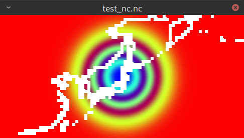
Here is a screenshot of the pressure data as viewed from ncview:

3. Save data to a netCDF file¶

Now save the newly crafted pressure data to a netCDF file on disk: